About shell elements | ||
| ||
Abaqus offers a wide variety of shell modeling options.
Conventional shell versus continuum shell
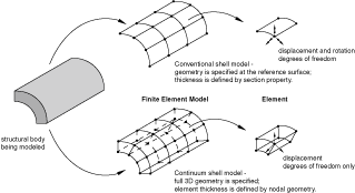
Shell elements are used to model structures in which one dimension, the thickness, is significantly smaller than the other dimensions. Conventional shell elements use this condition to discretize a body by defining the geometry at a reference surface. In this case the thickness is defined through the section property definition. Conventional shell elements have displacement and rotational degrees of freedom.
In contrast, continuum shell elements discretize an entire three-dimensional body. The thickness is determined from the element nodal geometry. Continuum shell elements have only displacement degrees of freedom. From a modeling point of view continuum shell elements look like three-dimensional continuum solids, but their kinematic and constitutive behavior is similar to conventional shell elements.
Figure 1 illustrates the differences between a conventional shell and a continuum shell element.
![]()
Conventions
The conventions that are used for shell elements are defined below.
Definition of local directions on the surface of a shell in space
The default local directions used on the surface of a shell for definition of anisotropic material properties and for reporting stress and strain components are defined in Conventions. You can define other directions by defining a local orientation (see Orientations), except for SAX1, SAX2, and SAX2T elements (Axisymmetric shell element library), which do not support orientations. A spatially varying local coordinate system defined with a distribution (Distribution definition) can be assigned to shell elements. For SAXA elements (Axisymmetric shell elements with nonlinear, asymmetric deformation) any anisotropic material definition must be symmetric with respect to the r–z plane at and .
In large-deformation (geometrically nonlinear) analysis these local directions rotate with the average rotation of the surface at that point. They are output as directions in the current configuration except in the shell elements in Abaqus/Standard that provide only large rotation but small strain (element types STRI3, STRI65, S4R5, S8R, S8RT, S8R5, S9R5—see Choosing a shell element), where they are output as directions in the reference configuration. Therefore, in geometrically nonlinear analysis, when displaying these directions or when displaying principal values of stress, strain, or section forces or moments in Abaqus/CAE, the current (deformed) configuration should be used except for the small-strain elements in Abaqus/Standard, for which the reference configuration should be used.
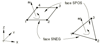
Positive normal definition for conventional shell elements
The “top” surface of a conventional shell element is the surface in the positive normal direction and is referred to as the positive (SPOS) face for contact definition. The “bottom” surface is in the negative direction along the normal and is referred to as the negative (SNEG) face for contact definition. Positive and negative are also used to designate top and bottom surfaces when specifying offsets of the reference surface from the shell's midsurface.
The positive normal direction defines the convention for pressure load application and output of quantities that vary through the thickness of the shell. A positive pressure load applied to a shell element produces a load that acts in the direction of the positive normal.
Three-dimensional conventional shells
For shells in space the positive normal is given by the right-hand rule going around the nodes of the element in the order that they are specified in the element definition. See Figure 2.
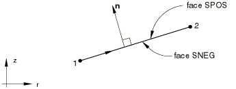
Axisymmetric conventional shells
For axisymmetric conventional shells (including the SAXA1n and SAXA2n elements that allow for nonsymmetric deformation) the positive normal direction is defined by a 90° counterclockwise rotation from the direction going from node 1 to node 2. See Figure 3.
Normal definition for continuum shell elements
Figure 4 illustrates the key geometrical features of continuum shells.
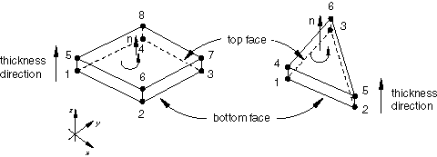
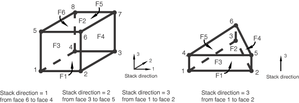
It is important that the continuum shells are oriented properly, since the behavior in the thickness direction is different from that in the in-plane directions. By default, the element top and bottom faces and, hence, the element normal, stacking direction, and thickness direction are defined by the nodal connectivity. For the triangular in-plane continuum shell element (SC6R) the face with corner nodes 1, 2, and 3 is the bottom face; and the face with corner nodes 4, 5, and 6 is the top face. For the quadrilateral continuum shell element (SC8R) the face with corner nodes 1, 2, 3, and 4 is the bottom face; and the face with corner nodes 5, 6, 7, and 8 is the top face. The stacking direction and thickness direction are both defined to be the direction from the bottom face to the top face. Additional options for defining the element thickness direction, including one option that is independent of nodal connectivity, are presented below.
Surfaces on continuum shells can be defined by specifying the face identifiers S1–S6 identifying the individual faces as defined in Continuum shell element library. Free surface generation can also be used.
Pressure loads applied to faces P1–P6 are defined similar to continuum elements, with a positive pressure directed into the element.
Defining the stacking and thickness direction
By default, the continuum shell stacking direction and thickness direction are defined by the nodal connectivity as illustrated in Figure 4. Alternatively, you can define the element stacking direction and thickness direction by either selecting one of the element's isoparametric directions or by using an orientation definition.
Defining the stacking and thickness direction based on the element isoparametric direction
You can define the element stacking direction to be along one of the element's isoparametric directions (see Figure 5 for element stack directions). The 8-node hexahedron continuum shell has three possible stacking directions; the 6-node in-plane triangular continuum shell has only one stack direction, which is in the element 3-isoparametric direction. The default stacking direction is 3, providing the same thickness and stacking direction as outlined in the previous section.
To obtain a desired thickness direction, the choice of the isoparametric direction depends on the element connectivity. For a mesh-independent specification, use an orientation-based method as described below.
Input File Usage
Use one of the following options to define the element stacking direction based on the element's isoparametric directions:
SHELL SECTION, STACK DIRECTION=n
SHELL GENERAL SECTION, STACK DIRECTION=n
where n = 1, 2, or 3.
Abaqus/CAE Usage
Use the following option to define the stacking direction based on the element's isoparametric directions if the continuum shell is defined using a composite layup:
Property module: Create Composite Layup: select Continuum Shell as the Element Type: Stacking Direction: Element direction 1, Element direction 2, or Element direction 3
Use the following option to define the stacking direction based on the element's isoparametric directions if the continuum shell is defined using a composite shell section:
: select regions: : Stacking Direction: Element isoparametric direction 1, Element isoparametric direction 2, or Element isoparametric direction 3
Defining the stacking and thickness direction based on an orientation definition
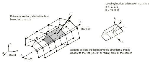
Alternatively, you can define the element stacking direction based on a local orientation definition. For shell elements the orientation definition defines an axis about which the local 1 and 2 material directions may be rotated. This axis also defines an approximate normal direction. The element stacking and thickness directions are defined to be the element isoparametric direction that is closest to this approximate normal (see Figure 6).
The pinched cylinder problem and LE3: Hemispherical shell with point loads illustrate the use of a cylindrical and spherical orientation system, respectively, to define the stack and thickness direction independent of nodal connectivity.
Input File Usage
Use one of the following options to define the element stacking direction based on a user-defined orientation:
SHELL SECTION, STACK DIRECTION=ORIENTATION, ORIENTATION=name
SHELL GENERAL SECTION, STACK DIRECTION=ORIENTATION,
ORIENTATION=name
Abaqus/CAE Usage
Use the following option to define the stacking direction based on a user-defined orientation if the continuum shell is defined using a composite layup:
Property module: Create Composite Layup: select Continuum Shell as the Element Type: Stacking Direction: Layup orientation
Use the following option to define the stacking direction based on a user-defined orientation if the continuum shell is defined using a composite shell section:
: select regions: : Stacking Direction: Normal direction of material orientation
Verifying the element stack and thickness direction
You can verify the element stack and thickness direction visually in Abaqus/CAE by either contouring the element section thickness or plotting the material axis. Generally, the in-plane dimensions are significantly larger than the element thickness. By contouring the shell section thickness, output variable STH, you can easily verify that all elements are oriented appropriately and have the correct thickness. If the element is oriented improperly, one of the in-plane dimensions will become the element section thickness, resulting in a discontinuous contour plot.
Alternatively, you can plot the material axis to verify that the 3-axis points in the desired normal direction. If the element is oriented improperly, one of the in-plane axes (either the 1- or 2-axis) would point in the normal direction.
Numbering of section points through the shell thickness
The section points through the thickness of the shell are numbered consecutively, starting with point 1. For shell sections integrated during the analysis, section point 1 is exactly on the bottom surface of the shell if Simpson's rule is used, and it is the point that is closest to the bottom surface if Gauss quadrature is used. For general shell sections, section point 1 is always on the bottom surface of the shell.
For a homogeneous section the total number of section points is defined by the number of integration points through the thickness. For shell sections integrated during the analysis, you can define the number of integration points through the thickness. The default is five for Simpson's rule and three for Gauss quadrature. For general shell sections, output can be obtained at three section points.
For a composite section the total number of section points is defined by adding the number of integration points per layer for all of the layers. For shell sections integrated during the analysis, you can define the number of integration points per layer. The default is three for Simpson's rule and two for Gauss quadrature. For general shell sections, the number of section points for output per layer is three.
Default output points
In Abaqus/Standard the default output points through the thickness of a shell section are the points that are on the bottom and top surfaces of the shell section (for integration with Simpson's rule) or the points that are closest to the bottom and top surfaces (for Gauss quadrature). For example, if five integration points are used through a single layer shell, output will be provided for section points 1 (bottom) and 5 (top).
In Abaqus/Explicit all section points through the thickness of a shell section are written to the results file for element output requests.