The Hertz contact problem | ||
| ||
ProductsAbaqus/StandardAbaqus/Explicit
Problem description
The Hertz contact problem studied consists of two identical, infinitely long cylinders pressed into each other. The solution quantities of most interest are the pressure distribution on the contacting area, the size of the contact area, and the stresses near the contact area. The material behavior is assumed to be linear elastic, and geometric nonlinearities are ignored. Therefore, the only nonlinearity in the problem is the contact constraint.
The cylinders in this example have a radius of 254 mm (10 in) and are elastic, with Young's modulus of 206 GPa (30 × 106 lb/in2) and Poisson's ratio of 0.3. Smooth contact (no friction) is assumed.
The contact area remains small compared to the radius of the cylinders, so the vertical displacements along the diametric chord of the cylinder that is parallel to the contact plane are almost uniform. This, together with the symmetry of the problem, requires only one-quarter of one cylinder to be modeled. Displacements are prescribed on the diametric cut parallel to the rigid plane to load the problem. For this example the nodes along the diametric cut are displaced vertically down by 10.16 mm (0.4 in). The total load per unit length of the cylinder can be obtained by summing the corresponding reaction forces on the cylinder or equivalently as the reaction force on the rigid body reference node.
For illustration, the problem is modeled in both two and three dimensions.
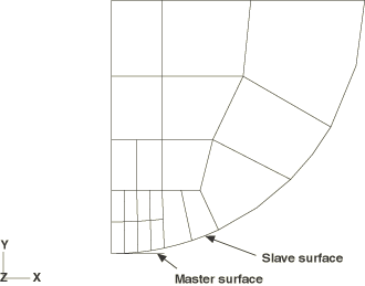
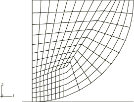
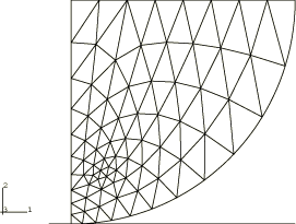
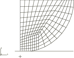
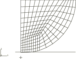
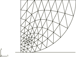
In the two-dimensional Abaqus/Standard case the quarter-cylinder is modeled with 20 8-node plane strain elements (see Figure 1). In the two-dimensional Abaqus/Explicit case the quarter-cylinder is modeled with either 171 4-node plane strain (CPE4R) elements (see Figure 5) or 130 6-node plane strain (CPE6M) elements (see Figure 6). In the three-dimensional cases a cylinder of unit thickness is modeled, with the out-of-plane displacements fixed on the two exterior faces of the model to impose the plane strain condition. The bulk of the cylinder is modeled in Abaqus/Standard with 16 20-node bricks; the remaining four elements that abut the surface where contact may occur are modeled with element type C3D27, which is a brick element that allows a variable number of nodes. This element is intended particularly for three-dimensional contact analysis. Element type C3D27 always has at least 21 nodes: the corner nodes, the midedge nodes, and one node at the element's centroid. The midface nodes may be omitted at the user's discretion. In this case the midface nodes on the surfaces where contact may occur are retained. The other midface nodes (on the element faces that are interior to the cylinder) are omitted, making those faces compatible with the 20-node bricks used in the remainder of the model. This use of 27-node brick elements is strongly recommended for three-dimensional contact problems in which second-order elements are used: it is almost essential for cases where partial contact may occur over element surfaces, as is the case in this example. The reason is that the interpolation on the surface of a quadratic element without a midface node is based on the four corner nodes and the four midedge nodes only and is, therefore, rather incomplete (it is not a product of Lagrange interpolations). Therefore, if a quadratic element is specified as part of the slave surface definition and there is no midface node on the contacting face, Abaqus/Standard will generate the midface node automatically and modify the element definition appropriately. In Abaqus/Explicit meshes with either C3D8R elements or C3D10M elements are used.
It is clearly advisable to refine the portion of the mesh near the expected contact region to predict the contact pressure and contact area accurately. This refinement is accomplished in Abaqus/Standard by using one of the default multi-point constraints provided for this purpose (General multi-point constraints). In Abaqus/Explicit a more refined mesh with mesh gradation is used.
To be consistent with the Hertz solution, geometric nonlinearities are neglected for all Abaqus/Explicit cases.
![]()
Contact modeling
Because of symmetry, the contact problem can be modeled as a deformable cylinder being pressed against a flat, rigid surface. Therefore, two contact surfaces are required: one (the slave surface in Abaqus/Standard) on the deformable cylinder and the other (the master surface in Abaqus/Standard) on the rigid body.
For illustrative purposes several different techniques are used to define the contacting surface pairs. The slave surface is defined by (1) grouping the free faces of elements in an element set that includes all elements in the region that potentially will come into contact (Abaqus defines the faces automatically), (2) specifying the faces of the elements (or the element sets) in the contact region, or (3) identifying the nodes on the deformable body in the contact region that may come into contact. The master surface is defined by (1) specifying the faces of the rigid elements (or element sets) used to define the rigid body or (2) defining the rigid surface with a surface definition and rigid body constraint. Any combination of these techniques can be used together.
By default, Abaqus uses a finite-sliding contact formulation for modeling the interaction between contact pairs. The contacting surfaces undergo negligible sliding relative to each other, which makes this problem a candidate for the small-sliding contact formulation. For a discussion of small- versus finite-sliding contact, see Contact formulations in Abaqus/Standard or Contact formulations for contact pairs in Abaqus/Explicit.
The surface contact formulation in Abaqus/Standard gives an accurate solution for the contact area and pressure distribution between the surfaces because of the choice of integration scheme used. Irons and Ahmad (1980) suggest a Gaussian integration rule for calculating self-consistent areas for surface boundary condition problems, which for second-order elements can lead to oscillating results for the pressure distribution on the surface. Oden and Kikuchi explain why this behavior occurs (1980) and present the remedy of using Simpson's integration rule instead. This technique is used in Abaqus/Standard, and no oscillations in the pressure distribution are found.
The default contact pair formulation in the normal direction in Abaqus/Standard is hard contact, which gives strict enforcement of contact constraints. Some standard analyses of this problem are conducted with both hard and augmented Lagrangian contact to demonstrate that the default penalty stiffness chosen by the code does not affect stress results significantly. The hard and augmented Lagrangian contact algorithms are described in Contact constraint enforcement methods in Abaqus/Standard.
The default contact pair formulation in Abaqus/Explicit is kinematic contact, which gives strict enforcement of contact constraints. (Note: the small-sliding contact option mentioned previously is available only with kinematic contact.) The explicit dynamic analyses of this problem are conducted with both kinematic and penalty contact to demonstrate that the penetration characteristic of the penalty method can affect stress results significantly in problems with displacement-controlled loading and purely elastic response. The kinematic and penalty contact algorithms are described in Contact constraint enforcement methods in Abaqus/Explicit.
![]()
Substructure Abaqus/Standard model
This type of contact problem is very suitable for analysis using the substructuring technique in Abaqus/Standard, since the only nonlinearity in the problem is the contact condition, which is quite local. The cylinder can be defined as a substructure and, thus, reduced to a small number of retained degrees of freedom on the surface where contact may occur or where boundary conditions may be changed. During the iterative solution for contact only these external degrees of freedom on the substructure appear in the equations, thus substantially reducing the cost per iteration. Once the local nonlinearity has been resolved, the solution in the cylinder is recovered as a purely linear response to the known displacements at these retained degrees of freedom. This technique is particularly effective in this case because the rigid surface is flat and there is no friction on the surface; therefore, only the displacement component normal to the surface needs to be retained in the nonlinear iterations.
All information that is relevant to the substructure generation must be given within the substructure generation step, including the degrees of freedom that will be retained. The substructure creation and usage cannot be included in the same input file. Only one substructure can be generated per input file. Any number of unit load cases can be defined for the substructure by using a substructure load case. Although this feature is not necessary in this example, it is used in one of the input files for verification purposes.
Substructures are introduced into an analysis model using elements, where the element number and nodes are defined for each usage of each substructure. Node and element numbers within a substructure and at the usage level are independent—the same node and element numbers can be reused in different substructures and on the usage level. It is also possible to refer to a substructure several times if the structure has identical sections. Thus, once a substructure has been created, it is used just as a standard element type.
![]()
Results and discussion
Results for the Abaqus/Standard and Abaqus/Explicit analyses are discussed in the following paragraphs.
Abaqus/Standard results
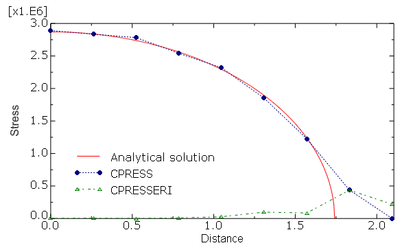
In spite of the rather coarse mesh, Figure 2 shows that the contact pressure between the cylinders predicted by the two-dimensional Abaqus/Standard model is in good agreement with the analytical distribution. The numerical solution is less accurate at the boundary of the contact patch where the contact pressure is characterized by a strong gradient. This aspect is also captured by the contact pressure error indicator. The only realistic way to improve the numerical solution would be to use a more detailed discretization. Almost identical results are obtained from the three-dimensional Abaqus/Standard model.
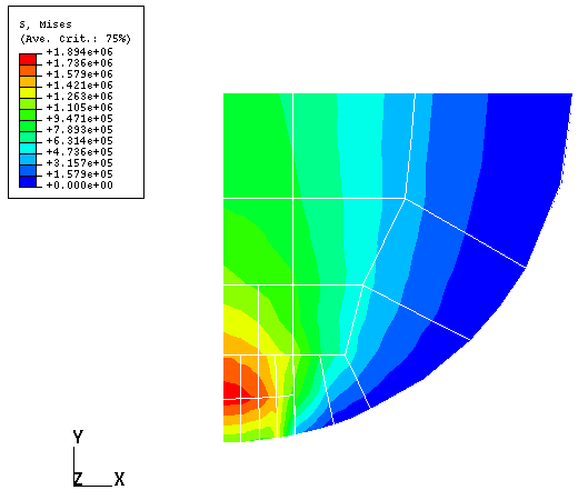
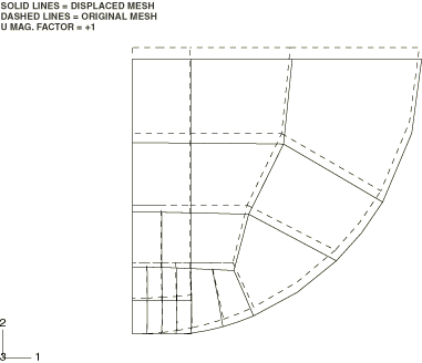
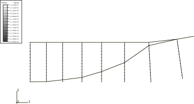
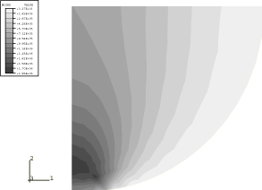
Figure 3 shows contours of Mises equivalent stress. This plot verifies that the highest stress intensity (where the material will yield first) occurs inside the body and not on the surface. Figure 4 shows the deformed configuration. In that figure the contacting surface of the cylinder appears to be curved downward because of the magnification factor used to exaggerate the displacements to show the results more clearly.
In this example substructuring reduces the computer time required for the job substantially because it allows the nonlinear contact problem to be resolved among a small number of active degrees of freedom. Substructuring involves considerable computational “overhead” because of the complex data management required. The reduced stiffness matrix coupling the retained degrees of freedom on a substructure is a full matrix. Thus, the method is not always as advantageous as this example would suggest. The use of substructures usually increases the analysis time in a purely linear analysis, unless a substructure can be used several times. In such cases the advantage of the method is that it allows a large analysis to be divided into several smaller analysis jobs, in each of which a substructure is created or substructures are used to build the next level of the analysis model.
Abaqus/Explicit results
The prescribed displacements on the diametric cut are ramped up over a relatively long time (.01 s) to minimize inertial effects. The displacements are then fixed for a short time (.001 s) to verify that the explicit dynamic results are truly quasi-static. Throughout the analysis the total kinetic energy is less than .1% of the total internal energy. In addition, the sum of the vertical reaction forces along the diametric cut closely matches the sum from the nodes in contact with the rigid body. These results indicate that the analysis can be accepted as quasi-static.
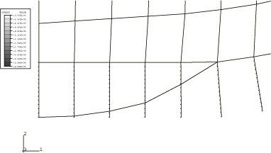
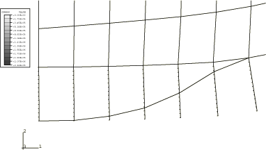
Figure 7 and Figure 8 show the contact pressures between the cylinders for the two-dimensional models using kinematic and penalty contact, respectively. The contact pressure distribution shows the classical elliptic distribution. The maximum pressure occurs at the symmetry plane and, for the kinematic contact analysis, is within 1% of the classical solution. However, the contact pressure is significantly lower when penalty contact is used because of the contact penetration. Almost identical results are obtained from the three-dimensional Abaqus/Explicit models.
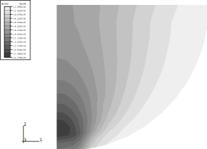
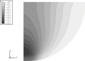
Figure 9 and Figure 10 show contours of Mises equivalent stress for kinematic and penalty contact, respectively. Again, the stress is significantly less with penalty contact than with kinematic contact. These plots verify that the highest stress intensity (where the material will yield first) occurs inside the body and not on the surface. Figure 11 and Figure 12 show the deformed configurations for the two types of contact enforcement; note the contact penetration in Figure 12.
In most cases kinematic contact and penalty contact will produce very similar results. However, there are exceptions, as this problem demonstrates. The user should be aware of the characteristics of both contact constraint methods, which are discussed in Contact constraint enforcement methods in Abaqus/Explicit. The kinematic contact method is better suited for this analysis because the penetrations associated with the penalty method influence the solution significantly. It is uncommon for these penetrations to be significant. Factors that tend to increase the significance of contact penetrations are: 1) displacement-controlled loading, 2) highly confined regions, 3) coarse meshes, and 4) purely elastic response. The penetrations can be reduced by increasing the penalty stiffness. However, increasing the penalty stiffness will tend to decrease the stable time increment and, thus, increase the analysis cost.
Figure 13 shows the contact pressure between the cylinders for a model meshed with CPE6M elements that uses kinematic contact enforcement. Figure 14 and Figure 15 show contours of Mises equivalent stress and the deformed configuration, respectively, for this analysis. The maximum contact pressure is again within 1% of the classical solution, and the distribution of Mises equivalent stress is very similar to that obtained with CPE4R elements and kinematic contact enforcement. Similar results are obtained using C3D10M elements.
![]()
Dynamic analysis in Abaqus/Standard
A simple dynamic example is created in Abaqus/Standard by giving the cylinder a uniform initial velocity with the contact conditions all open. This represents the experiment of dropping the cylinder onto a rigid, flat floor under a gravity field.
The impact algorithm used in Abaqus/Standard for dynamic contact is based on the assumption that, when any contact occurs, the total momentum of the bodies remains unchanged while the points that are contacting will acquire the same velocity instantaneously. In this example the cylinder contacts a rigid surface, which implies that each contacting point will suddenly have zero vertical velocity. This means that a compressive stress wave will emanate from the contacting point and will travel back into the cylinder. After some time this will cause the cylinder to rebound.
It is important to understand that the Abaqus/Standard dynamic contact algorithm is a “locally perfectly plastic impact” algorithm, as described above, which gives excellent results when it is used correctly. However, it is readily seen that, if the cylinder were modeled as a concentrated mass, with one vertical degree of freedom, the algorithm would imply that the cylinder stops instantaneously when it hits the rigid surface. In reality neither the cylinder nor the surface it hits are rigid: stress waves are started in each. Enough of this detail must be modeled for the results to be meaningful. In this example the cylinder itself is modeled in reasonable detail to capture at least the overall dynamic behavior. If the physical problem from which the example has been developed is that of two cylinders with equal and opposite velocities, this solution is probably useful. If the physical problem is that of a single cylinder hitting a flat surface, it may be necessary to include some elements to model the material below the surface (and the propagation of energy into that domain), unless that material is very dense so that this propagation can be neglected.
![]()
Input files
Abaqus/Standard input files
- hertzcontact_2d_relem.inp
Two-dimensional model with rigid elements.
- hertzcontact_2d_relem_auglagr.inp
Two-dimensional model with rigid elements and augmented Lagrangian contact.
- hertzcontact_2d_rsurf.inp
Two-dimensional model with a rigid surface.
- hertzcontact_2d_substr.inp
Analysis using substructuring.
- hertzcontact_2d_gen1.inp
Substructure generation referenced by the analysis hertzcontact_2d_substr.inp.
- hertzcontact_3d.inp
Three-dimensional problem.
- hertzcontact_3d_surf.inp
Three-dimensional problem, surface-to-surface approach.
- hertzcontact_3d_auglagr.inp
Three-dimensional problem with augmented Lagrangian contact.
- hertzcontact_3d_auglagr_surf.inp
Three-dimensional problem with augmented Lagrangian contact, surface-to-surface approach.
- hertzcontact_2d_dynamic.inp
Dynamic analysis.
- hertzcontact_2d_5inc.inp
Two-dimensional analysis with the step divided into five increments and the restart file saved.
- hertzcontact_2d_res.inp
A restart analysis from increment 2 of the previous job. These files are included to verify the restart capability with contact.
- hertzcontact_2d_substr_xnode.inp
Substructure analysis with additional nodes retained by moving the EQUATION definition to the global level.
- hertzcontact_2d_xnodes_gen1.inp
Substructure generation referenced by the analysis hertzcontact_2d_substr_xnode.inp.
- hertzcontact_2d_substr_sload.inp
Substructure analysis with the displacement loading applied using the SLOAD option.
- hertzcontact_2d_sload_gen1.inp
Substructure generation referenced by the analysis hertzcontact_2d_substr_sload.inp.
- hertzcontact_3d_substr.inp
Three-dimensional analysis using substructuring.
- hertzcontact_3d_gen1.inp
Substructure generation referenced by the analysis hertzcontact_3d_substr.inp.
- hertzcontact_3d_sub_only.inp
Generates the substructure only; outputs the matrix computed during the substructure generation, the substructure matrix, to a results file.
- hertzcontact_3d_sub_library.inp
Uses the substructure generated by the previous input file as a substructure library file; prints the substructure matrix to a results file after it has been read in as an element from the substructure file. The ELEMENT MATRIX OUTPUT option is used to output the matrix in this case.
- hertzcontact_3d_res.inp
Restart job of problem hertzcontact_3d_sub_library.inp. It is necessary to provide both the restart file and the substructure library file for this job.
- hertzcontact_3d_uel.inp
Uses the USER ELEMENT option to read in the substructure matrix output during its generation. This matrix is then used to complete the analysis.
- hertzcontact_3d_uel2.inp
Again uses the USER ELEMENT option to read in the substructure matrix. The same analysis is completed again with the matrix output during its use rather than during its generation.
- hertzcontact_2d_rsurf_unsym.inp
Two-dimensional model with rigid elements. This model uses the unsymmetric solver.
- hertzcontact_2d_rsurf_unsym_gen1.inp
Substructure generation referenced by the analysis hertzcontact_2d_rsurf_unsym.inp.
- hertzcontact_2d_symsub_unsym.inp
Uses a previously created symmetric substructure in a model that uses the unsymmetric solver.
- hertzcontact_2d_unsorted.inp
A substructure model with unsorted node sets and unsorted retained degrees of freedom.
- hertzcontact_2d_unsorted_gen1.inp
Substructure generation referenced by the analysis hertzcontact_2d_unsorted.inp.
- hertzcontact_cpe6m.inp
Two-dimensional problem with rigid elements and CPE6M elements.
- hertzcontact_cpe6m_auglagr.inp
Two-dimensional problem with rigid elements and CPE6M elements, augmented Lagrangian contact.
- hertzcontact_cpe6m_substr.inp
Two-dimensional problem with CPE6M elements using substructuring.
- hertzcontact_cpe6m_gen1.inp
Substructure generation referenced by the analysis hertzcontact_cpe6m_substr.inp.
- hertzcontact_cpe6m_dyn.inp
Two-dimensional dynamic analysis using CPE6M elements.
- hertzcontact_cpeg8.inp
Two-dimensional problem with rigid elements and CPEG8 elements.
- hertzcontact_2d_substr_cpeg8.inp
Two-dimensional problem with CPEG8 elements using substructuring.
- hertzcontact_2d_gen1_cpeg8.inp
Substructure generation referenced by the analysis hertzcontact_2d_substr_cpeg8.inp.
- hertzcontact_cpeg8_dyn.inp
Two-dimensional dynamic analysis using CPEG8 elements.
- hertzcontact_cpeg8_dyn_auglagr.inp
Two-dimensional dynamic analysis using CPEG8 elements and augmented Lagrangian contact.
- hertzcontact_c3d10m.inp
Three-dimensional problem using C3D10M elements.
- hertzcontact_c3d10m_auglagr.inp
Three-dimensional problem using C3D10M elements and augmented Lagrangian contact.
- hertzcontact_c3d10m_auglagr_res.inp
A restart analysis from increment 2 of the analysis hertzcontact_c3d10m_auglagr.inp.
- hertzcontact_c3d10m_substr.inp
Three-dimensional problem with C3D10M elements using substructuring.
- hertzcontact_c3d10m_gen1.inp
Substructure generation referenced by the analysis hertzcontact_c3d10m_substr.inp.
- hertzcontact_c3d10m_dyn.inp
Three-dimensional dynamic analysis using C3D10M elements.
- hertzcontact_substr45.inp
A substructure model where the substructure has been rotated through an angle of 45°. The EQUATION option is used during the substructure definition, and the TRANSFORM option is used at the usage level.
- hertzcontact_substr45_gen1.inp
Substructure generation referenced by the analysis hertzcontact_substr45.inp.
- hertzcontact_2d_cload.inp
A two-dimensional model in which the two cylinders are initially apart, and the deformation is produced by a point load instead of a displacement boundary condition. The CONTACT CONTROLS option with the STABILIZE parameter is used to prevent rigid body motion until contact is established.
- hertzcontact_2d_cload_auglagr.inp
An augmented Lagrangian contact model of the analysis hertzcontact_2d_cload.inp.
- hertzcontact_2d_kincoup.inp
Two-dimensional problem with the displacement applied through a KINEMATIC COUPLING reference node.
- hertzcontact_2d_substr_kincoup.inp
Two-dimensional problem using substructuring with the displacement applied to the top surface through the use of the KINEMATIC COUPLING option. The coupling reference node is one of the retained substructure nodes, providing a “handle” for displacing the model.
- hertzcontact_2d_kincoup_gen1.inp
Substructure generation referenced by the analysis hertzcontact_2d_substr_kincoup.inp.
- hertzcontact_2d_coupk.inp
Two-dimensional problem with the displacement applied to the top surface. The displacement of the top surface is controlled by a reference node through the use of the COUPLING and KINEMATIC options.
- hertzcontact_2d_coupk_substr.inp
Two-dimensional problem using substructuring. The displacement is applied to the top surface through the use of the COUPLING and KINEMATIC options. The coupling reference node is one of the retained substructure nodes, providing a “handle” for displacing the model.
- hertzcontact_2d_coupk_substrgen.inp
Substructure generation referenced by the analysis hertzcontact_2d_coupk_substr.inp.
- hertzcontact_2d_coupd_substr.inp
Two-dimensional problem using substructuring. The displacement is applied to the top surface through the use of the COUPLING and DISTRIBUTING options. The coupling reference node is one of the retained substructure nodes, providing a “handle” for displacing the model. The distributing weight factors are calculated automatically through the tributary surface area.
- hertzcontact_2d_coupd_substrgen.inp
Substructure generation referenced by the analysis hertzcontact_2d_coupd_substr.inp.
Note that in both hertzcontact_3d_uel.inp and hertzcontact_3d_uel2.inp the results file to be used is specified using the FILE parameter on the USER ELEMENT option.
Abaqus/Explicit input files
- hertz2d.inp
Two-dimensional kinematic contact model.
- hertz3d.inp
Three-dimensional kinematic contact model.
- hertz2d_pnlty.inp
Two-dimensional penalty contact model with default penalty stiffness.
- hertz3d_pnlty.inp
Three-dimensional penalty contact model with default penalty stiffness.
- hertz3d_gcont.inp
Three-dimensional general contact model with default penalty stiffness.
- hertz2d_pnlty_sc10.inp
Two-dimensional penalty contact model with the penalty stiffness equal to 10 times the default value.
- hertz3d_pnlty_sc10.inp
Three-dimensional penalty contact model with the penalty stiffness equal to 10 times the default value.
- hertz3d_sc10_gcont.inp
Three-dimensional general contact model with the penalty stiffness equal to 10 times the default value.
- hertz_c3d10m.inp
Three-dimensional kinematic contact model using 10-node quadratic modified tetrahedral elements.
- hertz_c3d10m_gcont.inp
Three-dimensional general contact model using 10-node quadratic modified tetrahedral elements.
- hertz_c3d10m_gcont_subcyc.inp
Three-dimensional general contact model using 10-node quadratic modified tetrahedral elements for the sole purpose of testing the performance of the subcycling.
- hertz_cpe6m.inp
Two-dimensional kinematic contact model using 6-node quadratic modified triangular elements.
![]()
References
- Techniques of Finite Elements, Ellis Horwood Ltd., Chichester England, 1980.
- Fifth Invitational Symposium of the Unification of Finite Elements, Finite Differences, Calculus of Variations, H. Kardestuncer, Editor, University of Connecticut at Storrs, 1980.
- Theory of Elasticity, Second edition, McGraw-Hill, New York, 1951.
![]()
Figures