Overview of Eulerian analyses

Pure Eulerian analysis is a finite element technique in which materials are allowed to flow across element boundaries in a rigid mesh. In the more traditional finite element formulation (also known as the Lagrangian technique), materials are closely associated with an element, and the materials move only with the deformation of the mesh. Because the element quality issues associated with a deformable mesh are not present in Eulerian analyses, the Eulerian technique can be very effective at treating problems involving very large deformations, material damage, or fluid materials. Eulerian analysis can be performed only in Dynamic, Explicit steps. For a detailed discussion of Eulerian capabilities and applications, refer to Eulerian analysis.

Context:

The techniques for modeling pure Eulerian analyses in Abaqus/CAE are very different than those used to model pure Lagrangian analyses. Most notably, instead of defining several parts and assembling them into a complete model, Eulerian models typically consist of a single Eulerian part. This part, which can be arbitrary in shape, represents the domain within which Eulerian materials can flow. The geometry of bodies in the model is not necessarily defined by the Eulerian part; instead, materials are assigned to different regions within the Eulerian part instance to define the body geometries.

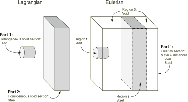
Figure 1 compares the same model created using Lagrangian and Eulerian techniques. In the Lagrangian model, two parts are modeled, and each part is assigned a unique section referencing a material. In the Eulerian model, a single Eulerian part is modeled and assigned an Eulerian section. The Eulerian section defines the materials that can be present within the part. Materials are then assigned to different regions within the instanced part; any region without a material assignment is treated as a void with no material properties.

Figure 1. Two bodies modeled using Lagrangian and Eulerian techniques.

The Eulerian analysis technique can be coupled with traditional Lagrangian techniques to extend the simulation functionality in Abaqus:

  • Arbitrary Lagrangian-Eulerian (ALE) adaptive meshing is a technique that combines features of Lagrangian and Eulerian analysis within the same part mesh. ALE adaptive meshing is typically used to control element distortion in Lagrangian parts undergoing large deformations, such as in a forming analysis. Most ALE adaptive meshing analyses can also be performed as pure Eulerian analyses, but some of the features associated with a Lagrangian mesh will be lost; for a more detailed comparison, see About ALE adaptive meshing.

  • Coupled Eulerian-Lagrangian (CEL) analysis allows Eulerian and Lagrangian bodies within the same model to interact. Coupled Eulerian-Lagrangian analysis is typically used to model the interactions between a solid body and a yielding or fluid material, such as a Lagrangian drill traveling through Eulerian soil or an Eulerian gas inflating a Lagrangian airbag. Eulerian-Lagrangian analysis is discussed in Assembling coupled Eulerian-Lagrangian models in Abaqus/CAE.

Viewing the results of Eulerian analyses requires some special techniques in the Visualization module. These techniques are discussed in detail in Viewing output from Eulerian analyses.

The procedure for creating Eulerian models in Abaqus/CAE involves the following general steps:

  1. In the Part module, create an Eulerian-type part that defines the geometric region within which Eulerian materials can flow. For more information, see Choosing the type of a new part.

  2. In the Part module, you may want to create partitions that represent the initial boundaries between different materials in the part. The partitions will affect the mesh of the part, and they are necessary only if you are assigning materials uniformly across a region. For more information about assigning materials in an Eulerian part, see Assigning materials to Eulerian part instances, and Defining a material assignment field.

  3. In the Property module, define the materials in the model.

  4. In the Property module, define and assign an Eulerian section for the model. The Eulerian section determines which materials can be present in the Eulerian part. The topology of the materials within the part will be defined in the Load module, as discussed in Step 7. For more information, see Creating Eulerian sections.

  5. In the Assembly module, create an instance of the Eulerian part.

  6. In the Step module, create a field output request for output variable EVF. This output is necessary to view the deformation of materials in an Eulerian model. For more detailed information, see Viewing output from Eulerian analyses.

  7. In the Load module, create a material assignment predefined field that defines the topology of materials in the initial configuration of the Eulerian part instance. For more information, see Assigning materials to Eulerian part instances, and Defining a material assignment field.

  8. In the Load module, define any loads or boundary conditions acting on the model. Because the mesh in an Eulerian part is rigid, traditional Lagrangian prescribed conditions do not move with the material deformations; loads and boundary conditions are imposed on any material that occupies (or moves into) the region to which the condition is prescribed. Zero-displacement boundary conditions can be used along the sides of an Eulerian part instance to prevent Eulerian material from entering or exiting the part. Boundary conditions and constraints based on nonzero nodal displacements are ignored in an Eulerian part instance; typically, velocity boundary conditions or predefined fields are used to prescribe initial motion in an Eulerian model. Specialized Eulerian boundary conditions can also be defined to control the flow of material across the boundaries of the Eulerian part (see Defining an Eulerian boundary condition). For more information about applying loads and boundary conditions to Eulerian models, see Boundary conditions.

  9. In the Mesh module, create a hexagonal mesh for the Eulerian part. EC3D8R elements are assigned to the mesh by default. After creating a regular mesh, you can trim any elements that are not expected to experience material flow to reduce the model size and improve performance of the analysis.

An example of a basic Eulerian model created in Abaqus/CAE is provided in Eulerian analysis of a collapsing water column. More complicated Eulerian modeling procedures, including complex material assignments and coupled Eulerian-Lagrangian interactions, are illustrated in Impact of a water-filled bottle.