About the element library | ||
| ||
Characterizing elements
Five aspects of an element characterize its behavior:
-
Family
-
Degrees of freedom (directly related to the element family)
-
Number of nodes
-
Formulation
-
Integration
Each element in Abaqus has a unique name, such as T2D2, S4R, C3D8I, or C3D8R. The element name identifies each of the five aspects of an element. For details on defining elements, see Element definition.
Family
Figure 1 shows the element families that are used most commonly in a stress analysis; in addition, continuum (fluid) elements are used in a fluid analysis. One of the major distinctions between different element families is the geometry type that each family assumes.
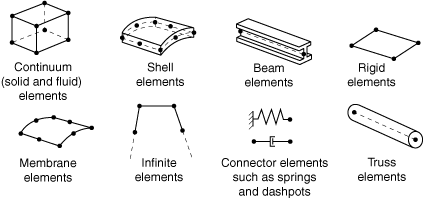
The first letter or letters of an element's name indicate to which family the element belongs. For example, S4R is a shell element, CINPE4 is an infinite element, and C3D8I is a continuum element.
Degrees of freedom
The degrees of freedom are the fundamental variables calculated during the analysis. For a stress/displacement simulation the degrees of freedom are the translations and, for shell, pipe, and beam elements, the rotations at each node. For a heat transfer simulation the degrees of freedom are the temperatures at each node; for a coupled thermal-stress analysis temperature degrees of freedom exist in addition to displacement degrees of freedom at each node. Heat transfer analyses and coupled thermal-stress analyses therefore require the use of different elements than does a stress analysis since the degrees of freedom are not the same. See Conventions for a summary of the degrees of freedom available in Abaqus for various element and analysis types.
Number of nodes and order of interpolation
Displacements or other degrees of freedom are calculated at the nodes of the element. At any other point in the element, the displacements are obtained by interpolating from the nodal displacements. Usually the interpolation order is determined by the number of nodes used in the element.
-
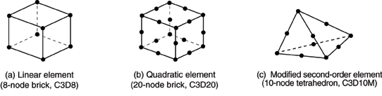
Elements that have nodes only at their corners, such as the 8-node brick shown in Figure 2(a), use linear interpolation in each direction and are often called linear elements or first-order elements.
-
In Abaqus/Standard elements with midside nodes, such as the 20-node brick shown in Figure 2(b), use quadratic interpolation and are often called quadratic elements or second-order elements.
-
Modified triangular or tetrahedral elements with midside nodes, such as the 10-node tetrahedron shown in Figure 2(c), use a modified second-order interpolation and are often called modified or modified second-order elements.
Typically, the number of nodes in an element is clearly identified in its name. The 8-node brick element is called C3D8, and the 4-node shell element is called S4R.
The beam element family uses a slightly different convention: the order of interpolation is identified in the name. Thus, a first-order, three-dimensional beam element is called B31, whereas a second-order, three-dimensional beam element is called B32. A similar convention is used for axisymmetric shell and membrane elements.
Formulation
An element's formulation refers to the mathematical theory used to define the element's behavior. In the Lagrangian, or material, description of behavior the element deforms with the material. In the alternative Eulerian, or spatial, description elements are fixed in space as the material flows through them. Eulerian methods are used commonly in fluid mechanics simulations. Abaqus/Standard uses Eulerian elements to model convective heat transfer. Abaqus/Explicit also offers multimaterial Eulerian elements for use in stress/displacement analyses. Adaptive meshing in Abaqus/Explicit combines the features of pure Lagrangian and Eulerian analyses and allows the motion of the element to be independent of the material (see About ALE adaptive meshing). All other stress/displacement elements in Abaqus are based on the Lagrangian formulation. In Abaqus/Explicit the Eulerian elements can interact with Lagrangian elements through general contact (see Eulerian analysis).
To accommodate different types of behavior, some element families in Abaqus include elements with several different formulations. For example, the conventional shell element family has three classes: one suitable for general-purpose shell analysis, another for thin shells, and yet another for thick shells. In addition, Abaqus also offers continuum shell elements, which have nodal connectivities like continuum elements but are formulated to model shell behavior with as few as one element through the shell thickness.
Some Abaqus/Standard element families have a standard formulation as well as some alternative formulations. Elements with alternative formulations are identified by an additional character at the end of the element name. For example, the continuum, beam, and truss element families include members with a hybrid formulation (to deal with incompressible or inextensible behavior); these elements are identified by the letter H at the end of the name (C3D8H or B31H).
Abaqus/Standard uses the lumped mass formulation for low-order elements; Abaqus/Explicit uses the lumped mass formulation for all elements. As a consequence, the second mass moments of inertia can deviate from the theoretical values, especially for coarse meshes.
In steady-state dynamic and frequency extraction procedures (see About dynamic analysis procedures), Abaqus/Standard uses a special projected mass matrix algorithm for the S3, S3R, S4, S4R, SC6R, SC8R, and S4R5 shell elements. As a consequence, slight differences may be observed in models that contain these elements when comparing results from steady-state dynamic and frequency extraction procedures to those of an implicit dynamic analysis.
Integration
Abaqus uses numerical techniques to integrate various quantities over the volume of each element, thus allowing complete generality in material behavior. Using Gaussian quadrature for most elements, Abaqus evaluates the material response at each integration point in each element. Some continuum elements in Abaqus can use full or reduced integration, a choice that can have a significant effect on the accuracy of the element for a given problem.
Abaqus uses the letter R at the end of the element name to label reduced-integration elements. For example, CAX4R is the 4-node, reduced-integration, axisymmetric, solid element.
Shell, pipe, and beam element properties can be defined as general section behaviors; or each cross-section of the element can be integrated numerically, so that nonlinear response associated with nonlinear material behavior can be tracked accurately when needed. In addition, a composite layered section can be specified for shells and, in Abaqus/Standard, three-dimensional bricks, with different materials for each layer through the section.
![]()
Combining elements
The element library is intended to provide a complete modeling capability for all geometries. Thus, any combination of elements can be used to make up the model; multi-point constraints (General multi-point constraints) are sometimes helpful in applying the necessary kinematic relations to form the model (for example, to model part of a shell surface with solid elements and part with shell elements or to use a beam element as a shell stiffener).
![]()
Heat transfer and thermal-stress analysis
In cases where heat transfer analysis is to be followed by thermal-stress analysis, corresponding heat transfer and stress elements are provided in Abaqus/Standard. See Sequentially coupled thermal-stress analysis for additional details.
![]()
Information available for element libraries
The complete element library in Abaqus is subdivided into a number of smaller libraries. Each library is presented as a separate section in this guide. In each of these sections, information regarding the following topics is provided where applicable:
-
conventions;
-
element types;
-
degrees of freedom;
-
nodal coordinates required;
-
element property definition;
-
element faces;
-
element output;
-
loading (general loading, distributed loads, foundations, distributed heat fluxes, film conditions, radiation types, distributed flows, distributed impedances, electrical fluxes, distributed electric current densities, and distributed concentration fluxes);
-
nodes associated with the element;
-
node ordering and face ordering on elements; and
-
numbering of integration points for output.
For element libraries that are available in both Abaqus/Standard and Abaqus/Explicit, individual element or load types that are available only in Abaqus/Standard are designated with an (S); similarly, individual element or load types that are available only in Abaqus/Explicit are designated with an (E). Element or load types that are available in Abaqus/Aqua are designated with an (A).
Most of the element output variables available for an element are discussed. Additional variables may be available depending on the material model or the analysis procedure that is used. Some elements have solution variables that do not pertain to other elements of the same type; these variables are specified explicitly.