About connectors

The analyst is often faced with modeling problems in which two different parts are connected in some way. Sometimes connections are simple, such as two panels of sheet metal spot welded together or a door connected to a frame with a hinge. In other cases the connection may impose more complicated kinematic constraints, such as constant velocity joints, which transmit constant spinning velocity between misaligned and moving shafts. In addition to imposing kinematic constraints, connections may include (nonlinear) force versus displacement (or velocity) behavior in their unconstrained relative motion components, such as a muscle force resisting the rotation of a knee joint in a crash-test occupant model. More complex connections may include the following:

• stopping mechanisms, which restrict the range of motion of an otherwise unconstrained relative motion;

• internal friction, such as the lateral force or moments on a bolt generating friction in the translation of the bolt along a slot;

• failure conditions, where excess force or displacement inside the connection causes the entire connection or a single component of relative motion to break free; and

• locking mechanisms that engage after some force or displacement criteria is met, such as a snap-fit connector or a falling-pin locking mechanism on a satellite deployment arm.

In many situations the connection can be actuated either through displacement or force control, such as a hydraulic piston or a gear-driven robot arm.

In Abaqus/Standard if the two parts being connected are rigid bodies, multi-point constraints cannot be used to connect the bodies at nodes other than the reference nodes, since multi-point constraints use degree-of-freedom elimination and the other nodes on a rigid body do not have independent degrees of freedom. In Abaqus/Explicit this restriction does not apply. See General multi-point constraints.

Connector elements in Abaqus provide an easy and versatile way to model these and many other types of physical mechanisms whose geometry is discrete (i.e., node-to-node), yet the kinematic and kinetic relationships describing the connection are complex.

In many instances connector elements perform functions similar to multi-point constraints (General multi-point constraints). However, in most cases multi-point constraints eliminate degrees of freedom at one of the nodes involved in the connection. This elimination has the advantage that the problem size is reduced; it has the disadvantage that output and other functionality provided with connector elements is not available. In addition, in Abaqus/Standard the degree of freedom elimination prevents the use of multi-point constraints between nodes without independent degrees of freedom (such as nodes on a rigid body whose degrees of freedom are dependent on the degrees of freedom at the reference node).

In contrast, connector elements do not eliminate degrees of freedom; kinematic constraints are enforced with Lagrange multipliers. These Lagrange multipliers are additional solution variables in Abaqus/Standard. The Lagrange multipliers provide constraint force and moment output. Since connector elements do not eliminate degrees of freedom, they can be used in many situations where multi-point constraints cannot be used or do not exist for the function required; for example, to connect two rigid bodies at nodes other than the reference node in Abaqus/Standard.

Multi-point constraints are more efficient than connector elements; and if the requirements of the analysis can be satisfied with multi-point constraints, they should be used in place of connector elements.

The following template shows the options used to define and activate the connector elements shown in Figure 1 and Figure 2. In the respective figures on the left is a schematic representation of a connection to be modeled; on the right is a representation of the equivalent finite element model. All options are discussed in detail in the following sections.

Figure 1. Simplified connector model of a shock absorber.

Figure 2. A pin-in-slot connection modeled with SLOT and CARDAN connection types.

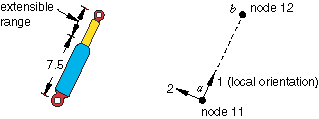
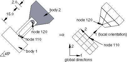
HEADING
...
ELEMENT, TYPE=CONN3D2, ELSET=shock
101, 11, 12
ELEMENT, TYPE=CONN3D2, ELSET=pininslot
1010, 110, 120
...
ORIENTATION, NAME=ori60
0.5, 0.866025, 0.0, -0.866025, 0.5, 0.0
ORIENTATION, NAME=ori45
0.707, 0.707, 0.0, -0.707, 0.707, 0.0
CONNECTOR SECTION, ELSET=shock, BEHAVIOR=sbehavior
revolute, slot
ori60,
...
CONNECTOR BEHAVIOR, NAME=sbehavior
CONNECTOR DAMPING, COMPONENT=1
1500.0
*CONNECTOR FRICTIONCONNECTOR LOCK, COMPONENT=3, LOCK=4
 , , -500.0, 500.0
CONNECTOR ELASTICITY, COMPONENT=4, NONLINEAR
-900., -0.7
   0.,  0.0
1250.,  0.7
CONNECTOR CONSTITUTIVE REFERENCE
 , , , 22.5,
CONNECTOR STOP, COMPONENT=1
7.5, 15.0
...
CONNECTOR FRICTION
0.34, 0.55,  0.0
0.34, 0.10,  0.45
FRICTION
.15 
...
CONNECTOR SECTION, ELSET=pininslot
cardan, slot
ori45,
CONNECTOR MOTION
pininslot, 4
pininslot, 5
...
STEP
...
CONNECTOR MOTION, TYPE=VELOCITY
pininslot, 6, 0.7854
...
CONNECTOR LOAD
pininslot, 1, 1000.0
...
END STEP