Applying SAE filtering to an X–Y data object | |||||||
|
| ||||||
Context:
The SAE filtering operation performs two-pass, zero phase shift, second-order Butterworth filtering. The SAE filtering classes that are allowed in Abaqus/CAE are 60, 100, 180, 600, and 1000, as defined in SAE Standard J211 (OCT88). The Visualization module in Abaqus/CAE uses the Signal Analysis Software obtained from the National Highway Traffic Safety Administration (NHTSA). For more information, see the documentation for the Signal Analysis Software installation kit on the NHTSA website (search for NVS Software Applications on http://www.nhtsa.gov/).
Abaqus/CAE provides the following two types of SAE filtering functions:
The general operator, , uses a general filtering class and can filter data for a user-specified cutoff frequency.
Class-specific operators filter for each of the five supported SAE filtering classes: , , , , and . Because they use a specific filtering class, these operators do not support specification of a cutoff frequency.
Your X–Y data object must have a constant time step for it to be filtered. If the time step is not constant, Abaqus/CAE computes additional points at constant intervals by interpolation. The constant time step for SAE filtering is defined by the smallest time step in the X–Y data object to be filtered.
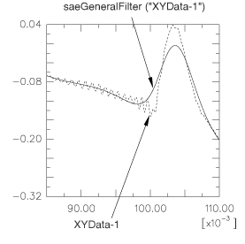
Figure 1 illustrates the type of X–Y plot that can be produced using the operation.
The function requires two arguments: the name of the X–Y data object (name) and the cutoff frequency (cutoffFrequency), which is the frequency above which the filter attenuates at least half of the input signal. The class-specific filters also require two arguments: the name of the X–Y data object (name) and the time scale factor (timeScaleFactor), which is a multiplier for the X-values of the data set being filtered. For example, a value of 1 indicates a time scale of seconds, and a value of 0.001 indicates a time scale of milliseconds.
A description of the optional arguments follows:
A symbolic constant specifying the method for computation of the projection and pre-charge to be applied at the start of the data signal (startCondition). Valid values for this argument are ZERO, which applies a constant projection and pre-charge of zero; CONSTANT, which applies a constant projection and pre-charge equal to the first data point in the X–Y data object; MIRROR, which applies a projection and pre-charge equivalent to reflecting the X–Y data object about a vertical line passing through the first data point; REVERSE_MIRROR, which applies a projection and pre-charge equivalent to reflecting the X–Y data object about both a vertical line and a horizontal line passing through the first data point; and TANGENTIAL, which applies a linear projection and pre-charge that is tangential to the first two data points. The default value is CONSTANT.
A symbolic constant specifying the method for computation of the projection and pre-charge to be applied at the end of the data signal (endCondition). Valid values for this argument are ZERO, which applies a constant projection and pre-charge of zero; CONSTANT, which applies a constant projection and pre-charge equal to the last data point in the X–Y data object; MIRROR, which applies a projection and pre-charge equivalent to reflecting the X–Y data object about a vertical line passing through the last data point; REVERSE_MIRROR, which applies a projection and pre-charge equivalent to reflecting the X–Y data object about both a vertical line and a horizontal line passing through the last data point; and TANGENTIAL, which applies a linear projection and pre-charge that is tangential to the last two data points. The default value is CONSTANT.
A symbolic constant that specifies the interpolation scheme (interpolation). Valid values for this argument are QUADRATIC, specifying a Lagrange second-order interpolation scheme; CUBIC_SPLINE, specifying a cubic spline interpolation scheme; and LINEAR, specifying a linear interpolation scheme. The default value is QUADRATIC.
The slope of the raw data curve leading up to the first data point (startslope). This argument's default value is 0.0 (for a level slope), and it is used only when interpolation=CUBIC_SPLINE.
The slope of the raw data curve continuing past the final data point (endslope). This argument's default value is 0.0 (for a level slope), and it is used only when interpolation=CUBIC_SPLINE.
A Boolean specifying whether a backward pass (backwardPass) is to be performed on the filtered data. The default value for this argument is True. When this argument is set to False, the endCondition argument is ignored.
Abaqus/CAE refers to the values in the table below to determine the cutoff frequency multiplier (CM) for the class-specific SAE filter operators.
| SAE class | Cutoff frequency multiplier (CM) |
|---|---|
| 60 | 100 |
| 100 | 165 |
| 180 | 300 |
| 600 | 1000 |
| 1000 | 1650 |
Abaqus/CAE then calculates the cutoff frequency using the cutoff frequency multiplier and the user-specified time scale factor (TSF), as follows: