Producing a contour plot of linear beam section stresses | ||||||
|
| |||||
Context:
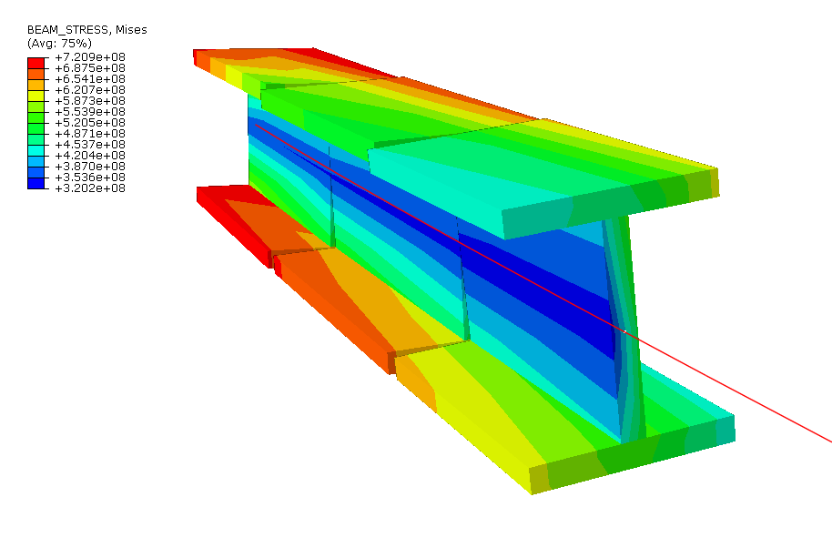
You can also create a contour plot that shows a more realistic stress distribution through the beam based on section force and section moment data, which Abaqus/CAE calculates using linear elastic solid mechanics theory. Figure 1 shows an example of beam stresses through an I-beam.
Beam stress contour plots are available only when the selected step and frame include data from the integrated output quantities SF (section force) and SM (section moment). Furthermore, these plots are available only for a subset of profiles in Abaqus/CAE:
Thin-walled box profiles
Thin-walled pipe profiles
Circular profiles
Rectangular profiles
I-shaped profiles
L-shaped profiles
T-shaped profiles
Contour plot display is unavailable for beam geometry in your model that uses any other profile or for tapered beam geometry.
Abaqus/CAE does not include beam element normals for eigenfrequency extraction in its calculations for beam cross section rendering, so you cannot visualize the torsional and out-of-plane modes for the beam elements in these plots. However, the torsional modes are calculated for the beam elements because the beam elements have torsional stiffness; this information is available in the data (.dat) file.
From the main menu bar, select and choose whether to plot the contours on the undeformed shape, the deformed shape, or both.
Tip: You can also produce a contour plot using the deformed  , undeformed
  , or superimposed
  contour tools in the toolbox.
The current viewport displays a customized contour plot of the specified field output variable at the specified step and frame of the current output database.
Abaqus automatically refreshes your contour plot each time you click in the step and frame selector, field output options, plot state–independent options, superimpose plot options (if applicable), or contour plot options dialog boxes.