Viewing and troubleshooting an optimization

When you submit an optimization process for analysis, Abaqus creates an output database (.odb) file for each design cycle of the optimization. The output database files are stored in the jobname\SAVE.odb directory. You must combine the separate output database files into a single output database file before you can view the optimization in the Visualization module. The behavior of the Visualization module depends on whether the output database file was created from a topology optimization, a shape optimization, a sizing optimization, or a bead optimization.

Topology optimization

When you view the results of a topology optimization, Abaqus/CAE automatically displays a view cut superimposed on the current view that represents the optimized design surface. The isosurface variable of the view cut is the normalized material property that the Optimization module uses to add or remove elements from the analysis. By default, Abaqus/CAE displays the view cut with the normalized material property set to 0.3. You can use the view cut manager to modify the value of the isosurface variable and to view the resulting boundary of the isosurface. Boundary conditions are not displayed while an optimization view cut is active. For more information, see Managing view cuts.

Shape optimization

When you view the results of a shape optimization, Abaqus/CAE displays the model in its optimized shape using the new position of the surface nodes.

Sizing optimization

When you view the results of a sizing optimization, Abaqus/CAE displays the shell model and the optimized shell thickness, which varies as the optimization progresses. (When you view the results of a nonoptimized analysis of a shell model, the shell thickness is read from the model data and does not change during the analysis.)

Bead optimization

When you view the results of a bead optimization, Abaqus/CAE displays the shell model in its optimized shape using the new position of the surface nodes.

After you combine the separate output database files into a single output database file, each design cycle in the optimization process appears as a frame in the output database, and you can open the Step/Frame dialog box to display the results from each design cycle. You can view the results of an optimization process while it is still in progress. As the optimization process moves toward completion, the lists of completed steps and frames are updated every time you close and reopen the Step/Frame dialog box. For more information, see Selecting a specific results step and frame, and Stepping through frames.

You can perform a time history animation of a deformed or contour plot and view the progress of the optimization as Abaqus attempts to satisfy the objective functions while respecting the constraints. For a topology optimization you can view the progressive removal of elements from the analysis and the resulting effect on the mechanical behavior of the model, such as the change in deformation or stress. Turning on translucency allows you to see the progression of the optimization through interior elements; for example, the removal of interior elements to create voids. For more information, see Changing the translucency. For a shape optimization you can view the incremental change in the position of the surface nodes as the optimization progresses; and, similar to a topology optimization, you can view the resulting effect on the mechanical behavior of the model.

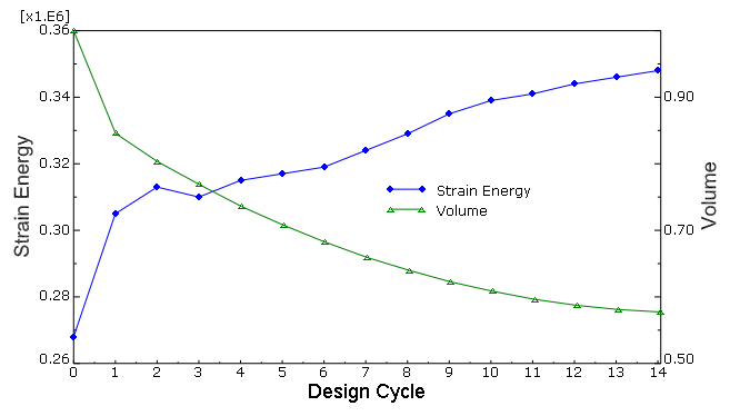
In addition, the optimization process writes data files (optimization_report.csv and optimization_status_all.csv) to the jobname directory that you can use to track the design variables. For example, you can create an X–Y plot showing how the objective functions and constraints change after each design cycle. The resulting plot indicates how the Optimization module tries to meet the specified objective functions while satisfying the constraints. You can use an X–Y plot of the objective functions and constraints as a diagnostic tool to view the progression of the optimization after each design cycle and to determine if the optimization is converging on a solution, as shown in Figure 1.

You can also view an X–Y plot showing how the objective function and constraints change after each design cycle by monitoring the progress of an optimization process from the optimization process manager. See Monitoring your optimization process, for more information.