Understanding view cuts | ||
| ||
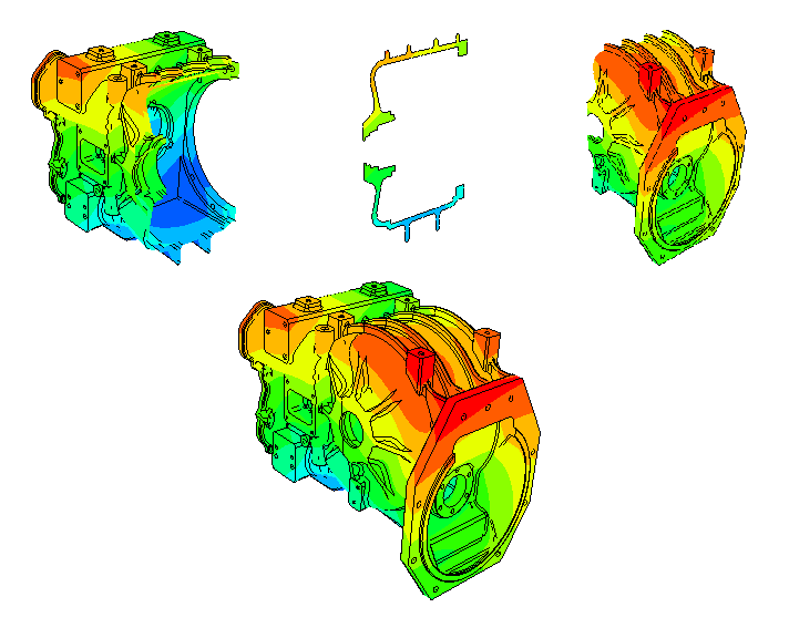
Figure 1 shows how a planar view cut can be used to cut through a contour plot of a gearbox model in the Visualization module.
- View cut shapes
-
You can create view cuts based on a plane. In the Visualization module you can also create view cuts based on the following shapes:
-
a cylinder,
-
a sphere, or
-
an isosurface corresponding to a constant value of a field variable or model attribute.
The types of shapes for view cut creation are illustrated in Figure 2.
Figure 2. View cuts based on planar, cylindrical, spherical, and isosurface shapes.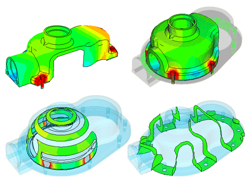
For isosurface cuts the result values are computed as described in Understanding how contour values are computed, for line- and banded-type contours. By default, Abaqus/CAE applies an averaging threshold of 100% for isosurface cuts to insure the continuous display of results at the cut location. You can apply an averaging threshold less than 100% by toggling off Override primary variable averaging when you create the isosurface cut. Abaqus/CAE then applies the averaging threshold specified in the Averaging options in the Result Options dialog box; for more information, see Controlling result averaging. Cuts along the X-, Y-, and Z-planes are created by default.
Note:
Isosurface view cuts offer slightly different functionality and behavior than isosurface-type contour plots. An isosurface view cut always reflects the results of the primary variable that was active when the view cut was created; you cannot change the variable for which an isosurface view cut displays results. By contrast, isosurface-type contour plots always display data from the currently selected primary variable for your session. Because each isosurface view cut is tied to a single variable, you can investigate the locations where two isosurface view cuts intersect if you display multiple isosurface view cuts that are based on different output variables.
-
- Displaying the cut section
-
To display the cut section of your model, you activate a cut and choose whether to display the model on the cut, above the cut, and/or below the cut, as illustrated in Figure 1. The cut itself is never visible. For planar cuts the portion of the model below the cut is defined as that part located on the negative side of the plane (relative to the orientation of the normal to the plane). For cylindrical and spherical cuts the portion of the model below the cut is defined as that part located at radii less than the radius of the cut shape. For an isosurface cut the portion of the model below the cut is defined as that part located at isovalues less than the specified isovalue. By default, Abaqus/CAE displays the model on and below the cut. In the Visualization module, you can display the model above the cut and the model below the cut at the same time; in all other modules, only one of these display options is available at a time.
- Plot options
-
You can select different plot options for the portions of the model below the cut, on the cut, and above the cut; for example, in Figure 2 some portions of the model are displayed with translucency activated, while others are displayed with no translucency.
- Displaying multiple view cuts (Visualization module only)
-
Only one cut can be active (used to display the model in the current viewport) at a time in modules other than the Visualization module; in the Visualization module, however, you can display multiple view cuts at once. In addition, in the Visualization module you can activate view cuts on undeformed, deformed, contour (texture-mapped only), symbol, or material orientation plots. For symbol and material orientation plots, Abaqus/CAE displays symbols and material orientation triads at all integration points for each element included in the view, even if the element is partially cut.
- Animation of view cuts (results data only)
-
Plots with an active view cut can be animated for output database data in the Visualization module; the view cut will be updated for each animation frame. View cuts cannot be activated on tessellated contour plots; swept, shrunk, or extruded plots; or highly refined plots (medium, fine, or extra fine).
- Results caching
-
By default, Abaqus/CAE caches the result values used to generate images of a cut model in memory to improve performance. However, you can disable results caching for cut fields to decrease memory usage if necessary; see Controlling results caching, for more information.
- Following the deformation
-
For plots of the deformed model, you can choose to have the cut follow the deformation; i.e., the cut surface will be calculated relative to a reference frame, and the cut deformation will match the deformation of the model.
- Repositioning view cuts
-
You can reposition cuts on your model: planar cuts can be rotated or translated, while the other cut shapes can only be translated.
- View Cut Manager
-
You can select a cut (either active or inactive) in the View Cut Manager to position, edit, copy, rename, or delete it. Selecting a cut in the manager is not the same as activating the cut. A cut can be both selected and active, unselected and active, or selected and inactive; and you can display or hide a free body cut for the currently displayed view cut if it is active. You can specify free body options that are common to all view cuts or that are specific to a particular view cut. Figure 3 shows an example of the information displayed in the view cut manager in the Visualization module; in other modules, the free body display and cut-specific options are not included in this dialog box.
Figure 3. The View Cut Manager dialog box in the Visualization module.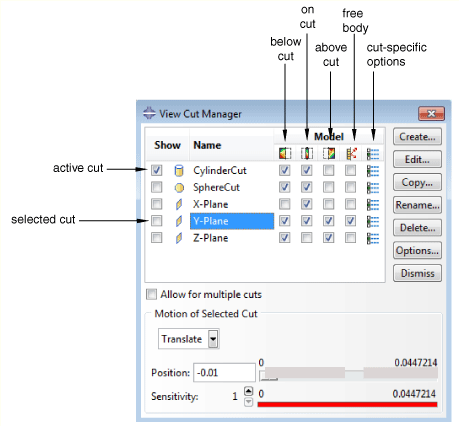
- Resultant forces and moments on view cuts (results data only)
-
For view cuts of output database data in the Visualization module you can also display the resultant forces and moments, and you can compute these values based on a display group, an element set, or the entire model. You can display the resultant force and moment on a view cut only for solid geometry, shell sections, or beam sections; for shell sections and beam sections the output database must include section force (SF) and section moment (SM) output for resultant forces and moments to be displayed. Abaqus/CAE does not support display of resultant forces and moments on view cuts for axisymmetric models. You can display the resultant force and moment on a view cut for any of the displayed view cuts in your session. Abaqus/CAE updates the resultant force and moment vectors and summation point as you reposition the view cut or animate the model.
By default, Abaqus/CAE displays vectors on the view cut only, showing the resultant force and moment across the view cut. However, you can also display a series of vectors that show resultant force and moment data at regular intervals in your model. This series of resultant force and moment vectors can run through the entirety of your model or within a user-specified region.
- XFEM-based view cut components (results data only)
-
Abaqus/CAE automatically creates and displays a view cut when you open an output database containing a crack calculated by the extended finite element method (XFEM). The view cut displays the model at the isosurface where the value of the signed distance function is zero, which corresponds with the surface of the XFEM crack. Boundary conditions are not displayed while an XFEM crack view cut is active.
The tools in the View Cut Manager operate as follows for XFEM cracks:
-
The below cut
 check box displays the entire model, except for the
XFEM crack.
check box displays the entire model, except for the
XFEM crack.
-
The on cut
 check box displays the isosurface where the value of the signed
distance function is zero, which corresponds with the surface of an
XFEM crack.
check box displays the isosurface where the value of the signed
distance function is zero, which corresponds with the surface of an
XFEM crack.
-
The above cut
 check box is not used by an
XFEM crack.
check box is not used by an
XFEM crack.
-
- Optimization-based view cut components (results data only)
-
Abaqus/CAE automatically creates and displays a view cut when you open an output database created by an optimization process, for both topology and shape optimizations. By default, the view cut displays the model at the isosurface where the value of the material property is zero, which corresponds with elements that have a density and stiffness close to zero and consequently play an insignificant role in the strength of the model. Boundary conditions are not displayed while an optimization view cut is active.
The tools in the View Cut Manager operate as follows for optimizations:
-
The below cut
check box displays the material that has a property less than
the value of the slider. By default, this is the material that is not
contributing to the strength of the model.
-
The on cut
check box displays the isosurface where the material has a
property equal to the value of the slider.
-
The above cut
check box displays the material that has a property greater than
the value of the slider. By default, this is the material that continues to
contribute to the strength of the model.
-
- Consideration for small faces
- A view cut may display inconsistent results if the area of one or more faces of the part is less than 1E–6 because faceting of such small faces is not possible.