Acoustic-structural interaction in an infinite acoustic medium | ||
| ||
ProductsAbaqus/StandardAbaqus/Explicit
Problem description
This benchmark problem is a simplified version of a characteristic problem in exterior acoustics: a thin shell structure immersed in a fluid. Since the intention here is only to test the effectiveness of the boundary conditions, the structure's purpose in this model is to introduce nontrivial dynamics in the acoustic mesh. In particular, the field incident on the radiating boundary should include significant spatial variation for the test to be meaningful.
The absorbing boundary conditions intended for three-dimensional applications are tested here in axisymmetric meshes. The two-dimensional elliptical and circular type radiation conditions are also applicable in three-dimensional analyses with radiating boundaries in the form of right-elliptic or right-circular cylinders.
Figure 1 shows the test mesh used for the circular and spherical boundary condition tests. On the inner radius of the mesh there is a circular structure of 4 units in radius consisting of shell elements in the axisymmetric case and beam elements in the two-dimensional case. The shells are connected to the acoustic domain with a tie constraint. The structure has stiffeners to disrupt the symmetry of the solution and to produce a nontrivial spatial variation in the pressure field incident on the absorbing boundary. Surrounding the structure is a fluid modeled with acoustic elements and terminated at the outer edge by the absorbing boundary conditions. The mesh shown uses an outer radius of eight units; it is stretched along the Y-axis by a factor of 1.2 for the elliptical and prolate spheroidal boundary condition tests.
Much larger meshes, 28 units in radius, are also run in both the axisymmetric and two-dimensional cases. The results from these meshes provide reference solutions against which to compare the results from the test meshes. Both steady-state and transient dynamic conditions are considered. The transient analyses are also performed using Abaqus/Explicit.
For tests of the acoustic infinite elements, the acoustic infinite elements are coupled directly to the structural model using a tie constraint. The center of the shell is used as the reference point for the acoustic infinite elements (see Acoustic, shock, and coupled acoustic-structural analysis). While in this case the acoustic infinite elements are coupled directly to the structural model, an alternative modeling strategy would involve defining an intermediate region comprising acoustic elements between the structure and the acoustic infinite elements. In certain situations the second approach may lead to improved accuracy.
The acoustic medium has a bulk modulus of 2.25E9 Pa and a density of 1000 (the properties of water). For the steady-state analyses the acoustic material has no volumetric drag. For the transient analyses a volumetric drag parameter is introduced with a numerical value equal to approximately 10% of the speed of sound. This value is not negligible in the sense of the approximation made in the derivation of this boundary condition (see Coupled acoustic-structural medium analysis); therefore, this case is a good test of the formulation.
![]()
Loading
The structure is excited in all cases with a concentrated load applied to degree of freedom 2 on the node at the free (innermost) end of the shell stiffener.
The absorbing boundary tests use nonreflecting boundary conditions to generate the necessary data automatically at the absorbing boundary. For the two-dimensional circular case and reference solutions and the spherical (axisymmetric) case and reference solutions, only the radius of the terminating circle or sphere need be specified to impose corresponding nonreflecting boundary conditions. In the two-dimensional elliptic case and the three-dimensional prolate spheroidal case, additional data need to be included to specify the size and orientation of the ellipse or spheroid.
For the Abaqus/Standard steady-state analyses using infinite elements, the infinite elements model radiation damping as well as the added mass effect, when coupled to the structural elements.
![]()
Results and discussion
The steady-state analyses are performed using the direct-solution steady-state dynamic procedure. The analyses are performed for two frequencies: the frequency corresponding to to test the effectiveness of the radiation boundary conditions, and the frequency corresponding to (in two dimensions) or (in three spatial dimensions) to test the limits of the acoustic mesh discretization (less challenging frequencies for the boundary conditions). Two steps are used. The impedance boundary condition is applied in the first step (for both frequencies). In the second step these impedances are removed and surfaces impedances of the same value are applied. The results with both options are identical.
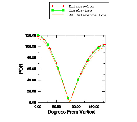
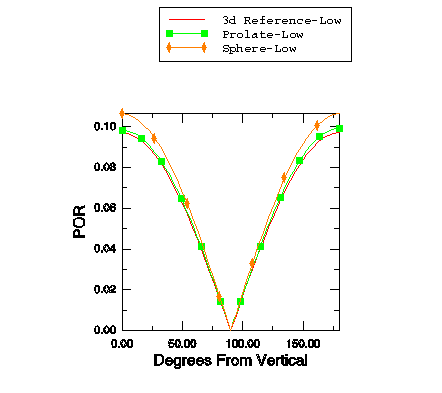
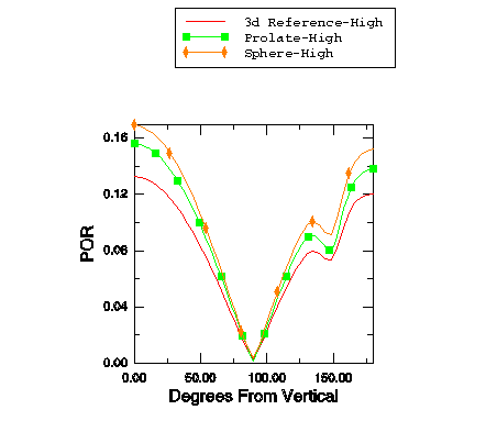
Each analysis shows good agreement between the reference solution and the solutions using the absorbing boundary conditions or the acoustic infinite elements on the smaller test meshes. The lower frequency is a more challenging test for the boundary conditions, particularly in two dimensions, where the boundary conditions are only asymptotic. Figure 2 through Figure 5 show the pressure amplitudes on the surface of the shell as a function of angular position. The angle is measured from the Y-axis, as shown in Figure 1. Each figure shows three curves; where differences between them are visible, the circular and elliptical condition solutions overlay the reference solution, and the spherical and prolate spheroidal conditions deviate by small amounts. The results from the acoustic infinite elements are similar.
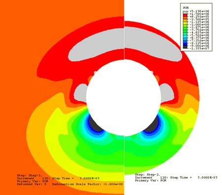
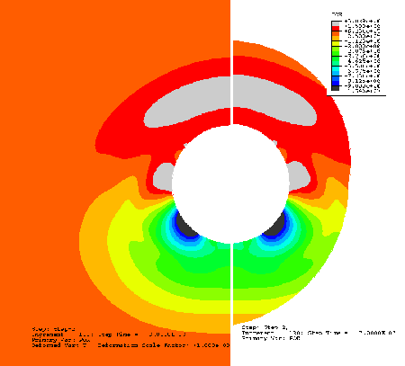
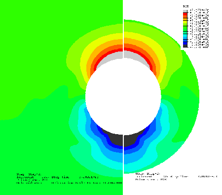
The transient analyses are performed with an excitation frequency of 100 Hz using two steps and a fixed time increment of 2.5 × 10⁻⁵ units, approximately one two-hundredth of the wavespeed. The analyses are run for 0.003 time units in the first step, where the impedance boundary condition is applied. This time period is long enough for the wave to reach the boundary of the test meshes. In the second step the simulation runs for another 0.003 units, this time with the boundary condition applied using a surface impedance. The total simulation time, 0.006 units, is not long enough for the wavefronts emanating from the structure to reach the boundary of the reference meshes, so the impedance conditions there do not play a role in the simulation. Figure 6 through Figure 9 show the pressure amplitudes in the acoustic domain at selected times. In each case the reference solution is on the left. Very good agreement is achieved in all cases; the three-dimensional boundary conditions perform slightly better, for reasons discussed in Coupled acoustic-structural medium analysis.
The Abaqus/Explicit transient analyses performed using acoustic infinite elements give very similar results to the Abaqus/Explicit transient analyses performed using nonreflecting boundary conditions. The test using two-dimensional acoustic infinite elements gives very similar results to the test using the circular radiation condition, while the test using axisymmetric acoustic infinite elements gives very similar results to the test using the spherical radiation condition. Figure 10 shows the pressure amplitudes on the surface of the shell at an angle of 90° to the vertical for the two-dimensional analysis (for a clear comparison the Abaqus/Standard transient analysis results are also included). The pressures are seen to match closely. The tests with acoustic infinite elements do not include any acoustic elements to model the fluid surrounding the structure. However, the additional computational cost due to the acoustic infinite elements offsets any savings obtained from not including the acoustic elements. For this example it was found that the acoustic infinite element analyses were about 12% more expensive than the corresponding analyses without acoustic infinite elements; i.e., with acoustic elements and nonreflecting boundary conditions.
![]()
Input files
Abaqus/Standard input files
- acoustic_bc_2dref.inp
-
Circular boundary condition, two-dimensional reference solution, steady state.
- acoustic_bc_acin2d2.inp
-
Linear, two-dimensional acoustic infinite elements, steady state.
- acoustic_bc_acin2d3.inp
-
Quadratic, two-dimensional acoustic infinite elements, steady state.
- acoustic_bc_acinax2.inp
-
Linear, axisymmetric acoustic infinite elements, steady state.
- acoustic_bc_acinax3.inp
-
Quadratic, axisymmetric acoustic infinite elements, steady state.
- acoustic_bc_circular.inp
-
Circular boundary condition, test mesh, steady state.
- acoustic_bc_circular_ams.inp
-
Circular boundary condition, test mesh, steady-state dynamic analysis following uncoupled AMS eigensolution.
- acoustic_bc_circular_ams_restart.inp
-
Steady-state dynamic analysis restarting from uncoupled AMS eigensolution.
- acoustic_bc_ellipse.inp
-
Elliptical boundary condition, test mesh, steady state.
- acoustic_bc_3dref.inp
-
Spherical boundary condition, three-dimensional reference solution, steady state.
- acoustic_bc_spherical.inp
-
Spherical boundary condition, test mesh, steady state.
- acoustic_bc_prolate.inp
-
Prolate spheroidal boundary condition, test mesh, steady state.
- acoustic_bc_2dref_trans.inp
-
Circular boundary condition, two-dimensional reference solution, transient.
- acoustic_bc_circular_trans.inp
-
Circular boundary condition, test mesh, transient.
- acoustic_bc_ellipse_trans.inp
-
Elliptical boundary condition, test mesh, transient.
- acoustic_bc_3dref_trans.inp
-
Spherical boundary condition, three-dimensional reference solution, transient.
- acoustic_bc_spherical_trans.inp
-
Spherical boundary condition, test mesh, transient.
- acoustic_bc_prolate_trans.inp
-
Prolate spheroidal boundary condition, test mesh, transient.
Abaqus/Explicit input files
- acoustic_bc_circular_xpl.inp
-
Circular boundary condition, test mesh.
- acoustic_bc_circular_xpl_subcyc.inp
-
Circular boundary condition, test mesh for the sole purpose of testing the performance of subcycling.
- acoustic_bc_ellipse_xpl.inp
-
Elliptical boundary condition, test mesh.
- acoustic_bc_spherical_xpl.inp
-
Spherical boundary condition, test mesh.
- acoustic_bc_prolate_xpl.inp
-
Prolate spheroidal boundary condition, test mesh.
- acoustic_bc_acin2d2_xpl.inp
-
Two-dimensional acoustic infinite elements, test mesh.
- acoustic_bc_acinax2_xpl.inp
-
Axisymmetric acoustic infinite elements, test mesh.
![]()
Figures