Finite-sliding interaction between a deformable and a rigid body

ProductsAbaqus/Standard

The finite-sliding rigid contact capability is implemented by means of a family of contact elements that Abaqus automatically generates based on the data associated with the user-specified contact pairs. At each integration point these elements construct a measure of overclosure (penetration of the point on the surface of the deforming body into the rigid surface) and measures of relative shear sliding. These kinematic measures are then used, together with appropriate Lagrange multiplier techniques, to introduce surface interaction theories (contact and friction). A library of interaction theories is provided in Abaqus—these may be thought of as a library of “surface constitutive models.” In this section we discuss only the kinematics of the interacting surfaces. The surface constitutive models are described in Mechanical Constitutive Theories.

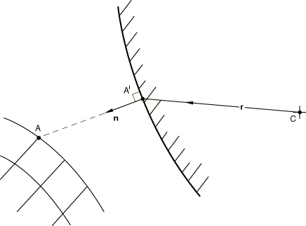
Let $A$ be a point on the deforming mesh, with current coordinates $x_{A}$ . Let $C$ be the “rigid body reference node”—the node that defines the position of the rigid body—with current coordinates $x_{C}$ . Let $A^{'}$ be the closest point on the surface of the rigid body to $A$ at which the normal to the surface of the rigid body, $n$ , passes through $A$ . Define $r$ as the vector from $C$ to $A^{'}$ . The geometry described by these quantities is shown in Figure 1.

Figure 1. Rigid surface interface geometry.

Let $h$ be the distance from $A^{'}$ to $A$ along $- n$ : the “overclosure” of the surfaces. From the definitions introduced above,

n h = - x_{A} + x_{C} + r .

Then if $h < - c$ there is no contact between the surfaces at $A$ , and no further surface interaction calculations need be done at this point. Here $c$ is the clearance below which contact occurs. For a “hard” surface $c = 0$ , but Abaqus/Standard also allows a “softened” surface to be introduced in which $c$ may be nonzero (although $c$ is usually very small compared to other dimensions). If $h \geq - c$ the surfaces are in contact. To enforce the contact constraint we will need the first variation of $h$ , $δ h$ , and its second variation, $d δ h$ . These quantities are now derived.

Let $S^{α}$ , $α = 1, 2$ be locally orthogonal, distance measuring surface coordinates on the surface at $A^{'}$ . The $S^{α}$ measure distance along the tangents $t_{α}$ to the surface at $A^{'}$ : these tangents are constructed according to the standard Abaqus convention for such tangents to a surface in space. As the point $A$ and the rigid body move, the projected point $A^{'}$ will move along. The movement consists of two parts: movement due to motion of the rigid body and motion relative to the body

δ x_{A^{'}} = δ x_{C} + {δ r |}_{γ_{α}} + {δ r |}_{ϕ_{C}} = δ x_{C} + δ ϕ_{C} \times r + t_{α} δ γ_{α},

where $δ γ_{α}$ is the “slip” of point $A^{'}$ . The normal $n$ will also change due to rotation of the rigid surface and due to slip along the surface

δ n = {δ n |}_{γ_{α}} + {δ n |}_{ϕ_{C}} = δ ϕ_{C} \times n + \frac{\partial n}{\partial S_{α}} δ γ_{α} .

The linearized form of the contact equation, thus, becomes

n δ h + h (δ ϕ_{C} \times n + \frac{\partial n}{\partial S_{α}} δ γ_{α}) = - δ x_{A} + δ x_{C} + δ ϕ_{C} \times r + t_{α} δ γ_{α} .

For “hard” contact $h = 0$ exactly, and for soft contact we will assume $h = 0$ as well. The linearized kinematic equation, thus, becomes

n δ h = - δ x_{A} + δ x_{C} + δ ϕ_{C} \times r + t_{α} δ γ_{α} .

This equation can be split into normal and tangential components, which yields the contact equation,

δ h = - n \cdot (δ x_{A} - δ x_{C}) + (r \times n) \cdot δ ϕ_{C},

and the slip equations,

δ γ_{α} = t_{α} \cdot (δ x_{A} - δ x_{C}) - (r \times t_{α}) \cdot δ ϕ_{C} .

To obtain the second variation of $h$ , it will again be assumed that $h = 0$ . In addition, it will be assumed that $d h = δ h = 0$ , which is accurate for relatively “hard” contact. It then directly follows that

n d δ h = d δ r,

and from the linearized kinematic equation follows

n d δ h = {d (δ ϕ_{C} \times r) |}_{γ_{β}} + {δ ϕ_{C} \times d r |}_{ϕ_{C}} + {d t |}_{γ_{β}} δ γ_{α} + {d t |}_{ϕ_{C}} δ γ_{α} + t_{α} d δ γ_{α},

where we have used $d δ x_{A} = d δ x_{C} = d δ ϕ_{C} = 0$ . The first term corresponds to a second-order variation on the vector $r$ for rigid body rotations around point $C$ and is given by (see Rotation variables):

{d (δ ϕ_{C} \times r) |}_{γ_{β}} = δ ϕ_{C} \cdot d ϕ_{C} r - \frac{1}{2} δ ϕ_{C} d ϕ_{C} \cdot r - \frac{1}{2} r \cdot δ ϕ_{C} d ϕ_{C} .

The second term in the expression for the second variation is obtained with the previously used expression for the “slip” along the surface:

{δ ϕ_{C} \times d r |}_{ϕ_{C}} = δ ϕ_{C} \times t_{α} d γ_{α} .

The third term follows from the expression for the rigid body rotation:

{d t |}_{γ_{β}} δ γ_{α} = d ϕ_{C} \times t_{α} δ γ_{α} .

Finally, the fourth term is obtained by differentiation along the surface coordinates:

{d t |}_{ϕ_{C}} δ γ_{α} = \frac{\partial t_{α}}{\partial S_{β}} d γ_{β} δ γ_{α} = δ γ_{α} κ_{α β} d γ_{β},

where

κ_{α β} = \frac{\partial t_{α}}{\partial S_{β}} = \frac{\partial t_{β}}{\partial S_{α}} = \frac{\partial^{2} r}{\partial S_{α} \partial S_{β}}

is the surface curvature matrix.

Substitution of the last four expressions in the expression for the second variation yields

n d δ h = δ ϕ_{C} \cdot d ϕ_{C} r - \frac{1}{2} δ ϕ_{C} d ϕ_{C} \cdot r - \frac{1}{2} r \cdot δ ϕ_{C} d ϕ_{C}

+ δ ϕ_{C} \times t_{α} d γ_{α} + d ϕ_{C} \times t_{α} δ γ_{α} + δ γ_{α} κ_{α β} d γ_{β} + t_{α} d δ γ_{α} .

As in the first variation, one can split the second variation into a normal and tangential components. For the normal component one finds

d δ h = (n \cdot r) δ ϕ_{C} \cdot d ϕ_{C} - \frac{1}{2} δ ϕ_{C} \cdot (nr + rn) \cdot d ϕ_{C}

+ δ ϕ_{C} \cdot (t_{α} \times n) d γ_{α} + d ϕ_{C} \cdot (t_{α} \times n) δ γ_{α} + δ γ_{α} n \cdot κ_{α β} d γ_{β}

and for the tangential components,

d δ γ_{α} = - (t_{γ} \cdot r) δ ϕ_{C} \cdot d ϕ_{C} + \frac{1}{2} δ ϕ_{C} \cdot (t_{γ} r + {rt}_{γ}) \cdot d ϕ_{C} + δ γ_{α} t_{γ} \cdot κ_{α β} d γ_{β} .

The expression involving $κ_{α β}$ can be simplified somewhat. Observe that $n \cdot t_{α} = 0$ ; hence,

n \cdot κ_{α β} = n \cdot \frac{\partial t_{α}}{\partial S_{β}} = - t_{α} \cdot \frac{\partial n}{\partial S_{β}} = t_{β} \cdot \frac{\partial n}{\partial S_{α}} .

Similarly

t_{γ} \cdot κ_{α β} = t_{γ} \cdot \frac{\partial t_{α}}{\partial S_{β}} = - t_{α} \cdot \frac{\partial t_{γ}}{\partial S_{β}} .

If the local surface coordinate system is created by projection of a tangential Cartesian $X$ – $Y$ system onto the surface, it is readily established that the last terms vanish. Hence, we will assume that the last term in the second variation is zero. The final result is obtained by substitution of the expressions for the first-order variation of the slip in the expressions for the second variation. After some reordering and with $κ_{α β} \equiv n \cdot κ_{α β}$ this furnishes

d δ h = (δ x_{A} - δ x_{C}) \cdot t_{α} κ_{α β} t_{β} \cdot (d x_{A} - d x_{C})

+ (δ x_{A} - δ x_{C}) \cdot (t_{α} κ_{α β} (t_{β} \times r) + t_{α} (t_{β} \times n)) \cdot d ϕ_{C}

+ δ ϕ_{C} \cdot ((t_{α} \times r) κ_{α β} t_{β} + (t_{α} \times n) t_{β}) \cdot (d x_{A} - d x_{C})

+ δ ϕ_{C} \cdot (t_{α} \times r) κ_{α β} (t_{β} \times r) \cdot d ϕ_{C}

+ (n \cdot r) δ ϕ_{C} \cdot d ϕ_{C} - \frac{1}{2} δ ϕ_{C} \cdot (nr + rn) \cdot d ϕ_{C}

d δ γ_{α} = - (t_{α} \cdot r) δ ϕ_{C} \cdot d ϕ_{C} + \frac{1}{2} δ ϕ_{C} \cdot (t_{α} r + {rt}_{α}) \cdot d ϕ_{C} .

The first two terms of the expression for $d δ h$ will only need to be included if slip occurs, whereas the expression for $d δ γ_{α}$ only needs to be taken into account if frictional forces are transmitted.

For dynamic applications we need the velocity and acceleration terms $\dot{h}$ and $\ddot{h}$ to calculate impact forces and impulses correctly. These terms are

\dot{h} = - n \cdot ({\dot{x}}_{A} - {\dot{x}}_{C} - {\dot{ϕ}}_{C} \times r)

(this is the same form as the first variation of $h$ ); and

\begin{matrix} \ddot{h} = & - n \cdot ({\ddot{x}}_{A} - {\ddot{x}}_{C} - {\ddot{ϕ}}_{C} \times r) + n \cdot {\dot{ϕ}}_{C} r \cdot {\dot{ϕ}}_{C} - n \cdot r {\dot{ϕ}}_{C} \cdot {\dot{ϕ}}_{C} \\ - ({\dot{x}}_{A} - {\dot{x}}_{C} - {\dot{ϕ}}_{C} \times r) \cdot ({\dot{ϕ}}_{C} \times n + \frac{\partial n}{\partial S^{α}} t_{α} \cdot ({\dot{x}}_{A} - {\dot{x}}_{C} - {\dot{ϕ}}_{C} \times r)) . \end{matrix}