Modifications to the model

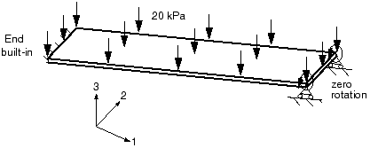
You will now reanalyze the plate in Abaqus/Standard to include the effects of geometric nonlinearity. The results from this analysis will allow you to determine the importance of geometrically nonlinear effects and, therefore, the validity of the linear analysis.

If you wish, you can follow the guidelines at the end of this example to extend the simulation to perform a dynamic analysis using Abaqus/Explicit.

Abaqus provides scripts that replicate the complete analysis model for this problem. Run one of these scripts if you encounter difficulties following the instructions given below or if you wish to check your work. Scripts are available in the following locations:

• A Python script for this example is provided in Nonlinear skew plate. Instructions on how to fetch the script and run it within Abaqus/CAE are given in Example Files.

• A plug-in script for this example is available in the Abaqus/CAE Plug-in toolset. To run the script from Abaqus/CAE, select Plug-insAbaqusGetting Started; highlight Nonlinear skew plate; and click Run. For more information about the Getting Started plug-ins, see Running the Getting Started with Abaqus examples.

Open the model database file SkewPlate.cae. Copy the model named Linear to a model named Nonlinear.

For the Nonlinear skew plate model, you will include nonlinear geometric effects as well as change the output requests.

Defining the step

In the Model Tree, double-click the Apply Pressure step underneath the Steps container to edit the step definition. In the Basic tabbed page of the Edit Step dialog box, toggle on Nlgeom to include geometric nonlinearity effects, and ensure the time period for the step is set to 1.0. In the Incrementation tabbed page, set the initial increment size to 0.1. The default maximum number of increments is 100; Abaqus may use fewer increments than this upper limit, but it will stop the analysis if it needs more.

You may wish to change the description of the step to reflect that it is now a nonlinear analysis step.

Output control

In a linear analysis Abaqus solves the equilibrium equations once and calculates the results for this one solution. A nonlinear analysis can produce much more output because results can be requested at the end of each converged increment. If you do not select the output requests carefully, the output files become very large, potentially filling the disk space on your computer.

As noted earlier, output is available in four different files:

• the output database (.odb) file, which contains data in a neutral binary format necessary to postprocess the results with Abaqus/CAE;

• the data (.dat) file, which contains printed tables of selected results (available only in Abaqus/Standard);

• the restart (.res) file, which is used to continue the analysis; and

• the results (.fil) file, which is used with third-party postprocessors.

Only the output database (.odb) file is discussed here. If selected carefully, data can be saved frequently during the simulation without using excessive disk space.

Open the Field Output Requests Manager. On the right side of the dialog box, click Edit to open the field output editor. Remove the field output requests defined for the linear analysis model, and specify the default field output requests by selecting Preselected defaults under Output Variables. This preselected set of output variables is the most commonly used set of field variables for a general static procedure.

To reduce the size of the output database file, write field output every second increment. If you were simply interested in the final results, you could either select Last increment or set the frequency at which output is saved equal to a large number. Results are always stored at the end of each step, regardless of the value specified; therefore, using a large value causes only the final results to be saved.

The history output request for the displacements of the nodes at the midspan can be kept from the previous analysis. You will explore these results using the X–Y plotting capability in the Visualization module.

Running and monitoring the job

Create a job for the Nonlinear model named NlSkewPlate, and give it the description Nonlinear Elastic Skew Plate. Remember to save your model in a new model database file.

Submit the job for analysis, and monitor the solution progress. If any errors are encountered, correct them; if any warning messages are issued, investigate their source and take corrective action as necessary.

Figure 2 shows the contents of the Job Monitor for this nonlinear skew plate simulation.

Figure 2. Job Monitor: nonlinear skew plate analysis.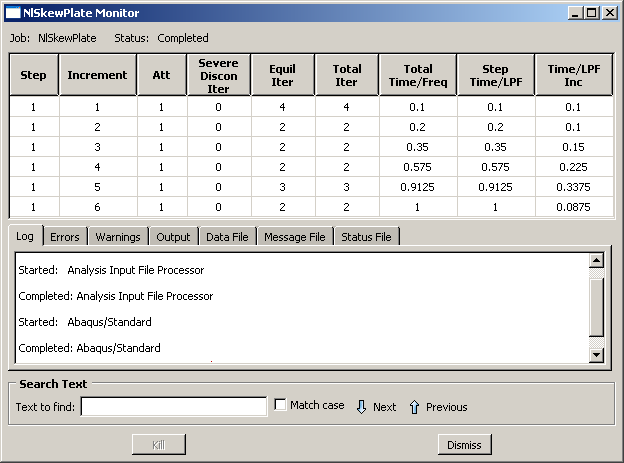

The first column shows the step number—in this case there is only one step. The second column gives the increment number. The sixth column shows the number of iterations Abaqus/Standard needed to obtain a converged solution in each increment; for example, Abaqus/Standard needed four iterations in increment 1. The eighth column shows the total step time completed, and the ninth column shows the increment size ($\mathrm{\Delta }T$).

This example shows how Abaqus/Standard automatically controls the increment size and, therefore, the proportion of load applied in each increment. In this analysis Abaqus/Standard applied 10% of the total load in the first increment: you specified $\mathrm{\Delta }{T}_{initial}$ to be 0.1 and the step time to be 1.0. Abaqus/Standard needed four iterations to converge to a solution in the first increment. Abaqus/Standard only needed two iterations in the second increment, so it automatically increased the size of the next increment by 50% to $\mathrm{\Delta }T$ = 0.15. Abaqus/Standard also increased $\mathrm{\Delta }T$ in both the fourth and fifth increments. It adjusted the final increment size to be just enough to complete the analysis; in this case the final increment size was 0.0875.