Calculation of phreatic surface in an earth dam | ||
| ||
ProductsAbaqus/Standard
Boundary conditions
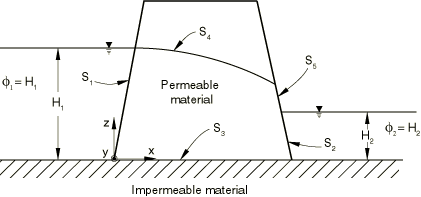
A typical dam is shown in Figure 1. We consider fluid flow only: deformation of the dam is ignored. Thus, although we use the fully coupled pore fluid flow-deformation elements, all displacement degrees of freedom are prescribed to be zero. A more general analysis would include stress and deformation of the dam.
The upstream face of the dam (surface in Figure 1) is exposed to water in the reservoir behind the dam. Since Abaqus uses a total pore pressure formulation, the pore pressure on this face must be prescribed to be , where is the elevation of the water surface, z is elevation, g is the gravitational acceleration, and is the mass density of the water. (, the weight density of the water, must be given as the value of the specific weight of the wetting fluid as part of the definition of material permeability.) Likewise, on the downstream face of the dam (surface in Figure 1),
The bottom of the dam (surface ) is assumed to rest on an impermeable foundation. Since the natural boundary condition in the pore fluid flow formulation provides no flow of fluid across a surface of the model, no further specification is needed on this surface.
The phreatic surface in the dam, , is found as the locus of points at which the pore fluid pressure, , is zero. Above this surface the pore fluid pressure is negative, representing capillary tension causing the fluid to rise against the gravitational force and creating a capillary zone. The saturation associated with particular values of capillary pressure for absorption and exsorption of fluid from the porous medium is a physical property of the material and is defined in the absorption/exsorption behavior under partially saturated flow conditions.
A special boundary condition is needed if the phreatic surface reaches an open, freely draining surface, as indicated on surface in Figure 1. In such a case the pore fluid can drain freely down the face of the dam, so = 0 at all points on this surface below its intersection with the phreatic surface. Above this point 0, with its particular value depending on the solution. This example is specifically chosen to include this effect to illustrate the use of the Abaqus drainage-only flow boundary condition.
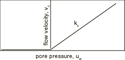
This drainage-only flow condition consists of prescribing the flow velocity on the freely draining surface in a way that approximately satisfies the requirement of zero pore pressure on the completely saturated portion of this surface (Pagano, 1997). The flow velocity is defined as a function of pore pressure, as shown in Figure 2. For negative pore pressures (those above the phreatic surface) the flow velocity is zero—the proper natural boundary condition. For positive pore pressures (those below the phreatic surface) the flow velocity is proportional to the pore pressure value. When this proportionality coefficient, , is large compared to —where k is the permeability of the medium, is the specific weight of the fluid, and c is a characteristic length scale—the requirement of zero pore pressure on the free-drainage surface below the phreatic surface will be satisfied approximately. The drainage-only seepage coefficient in this model is specified as 10−1 m3/Nsec. This value is roughly 105 times larger than the characteristic value, , based on the material properties listed below and an element length scale 10−1 m. This condition is prescribed using a pore fluid flow definition with the drainage-only flow type label (QnD) as shown in phreaticsurf_cpe8rp.inp.
![]()
Geometry and model
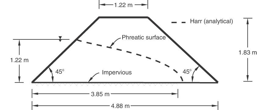
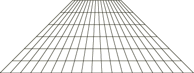
The geometry of the particular earth dam considered is shown in Figure 3. This case is chosen because an analytical solution is available for comparison (Harr, 1962). The dam is filled to two-thirds of its height. Only a part of its base is impermeable. Since the dam is assumed to be long, we use CPE8RP coupled pore pressure/displacement plane strain elements (the mesh is shown in Figure 4). In addition, input files containing element types CPE4P and CPE6MP are included for verification purposes. Additional input files are included to demonstrate the use of contact pairs, tie constraints, and solution transfer capabilities in coupled pore pressure-displacement analyses.
![]()
Material
The permeability of the fully saturated earth of which the dam is made is 0.2117 × 10⁻³ m/sec. The default assumption is used for the partially saturated permeability: that it varies as a cubic function of saturation, decreasing from the fully saturated value to a value of zero at zero saturation. The specific weight of the water is 10 kN/m3. The capillary action in the dam is defined by a single absorption/exsorption curve that varies linearly between a negative pore pressure of 10 kN/m2 at a saturation of 0.05 and zero pore pressure at fully saturated conditions. This is not a very realistic model of physical absorption/exsorption behavior, but this will not affect the results of the steady-state analysis significantly insofar as the location of the phreatic surface is concerned. Accurate definition of this behavior would be required if definition of the capillary zone created by filling and emptying the dam at given rates were needed.
The initial void ratio of the earth material is 1.0. The initial conditions for pore pressure and saturation are assumed to be those corresponding to the dam being fully saturated to the upstream water level: the initial saturation is, therefore, 1.0; and the initial pore pressures vary between zero at the water level and a maximum value of 12.19 kN/m2 at the base of the dam.
![]()
Loading and controls
The weight of the water is applied by GRAV loading, and the upstream and downstream pore pressures are prescribed as discussed above. A steady-state, coupled pore fluid diffusion/stress analysis is performed in five increments to allow Abaqus to resolve the high degree of nonlinearity in the problem.
![]()
Results and discussion
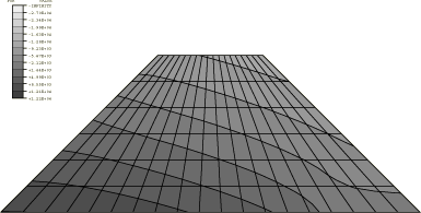
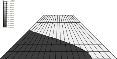
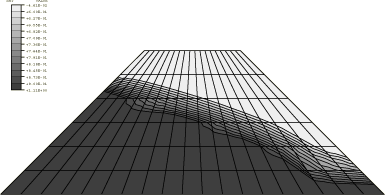
The steady-state contours of pore pressure are shown in Figure 5. The upper-right part of the dam shows negative pore pressures, indicating that it is partly saturated or dry. The phreatic surface is best shown in Figure 6, where we have chosen to draw the contours in the vicinity of zero pore pressure. This phreatic surface compares well with the analytical phreatic surface calculated by Harr (1962), shown in Figure 2. Figure 7 shows contours of saturation that indicate a region of fully saturated material under the phreatic zone and decreasing saturation in and above the phreatic zone.
![]()
Input files
- phreaticsurf_cpe8rp.inp
Phreatic surface calculation (element type CPE8RP).
- phreaticsurf_cpe4p.inp
Element type CPE4P.
- phreaticsurf_cpe6mp.inp
Element type CPE6MP.
- phreaticsurf_cpe4p_contactpair.inp
Element type CPE4P using the CONTACT PAIR option.
- phreaticsurf_cpe4p_mapsolution.inp
MAP SOLUTION continuation of thephreaticsurf_cpe4p_contactpair.inp analysis.
- phreaticsurf_cpe4p_tie.inp
Element type CPE4P using the TIE option.
![]()
References
- Groundwater and Seepage, McGraw-Hill, New York, 1962.
- “Steady State and Transient Unconfined Seepage Analyses for Earthfill Dams,” Abaqus Users' Conference, Milan, pp. 557–585, 1997.
![]()
Figures