Upsetting of a cylindrical billet: coupled temperature-displacement and adiabatic analysis | ||
| ||
ProductsAbaqus/StandardAbaqus/Explicit
Geometry and model
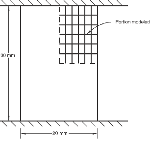
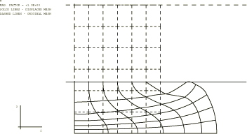
The specimen is shown in Figure 1: a circular billet, 30 mm long, with a radius of 10 mm, compressed between flat, rough, rigid dies. All surfaces of the billet are assumed to be fully insulated: this thermal boundary condition is chosen to maximize the temperature rise.
The finite element model is axisymmetric and includes the top half of the billet only since the middle surface of the billet is a plane of symmetry. In Abaqus/Standard elements of type CAX8RT, 8-node quadrilaterals with reduced integration that allow for fully coupled temperature-displacement analysis, are used. A regular mesh with six elements in each direction is used, as shown in Figure 1. In addition, the billet is modeled with CAX4RT elements in a 12 × 12 mesh for both Abaqus/Standard and Abaqus/Explicit analyses.
The contact between the top and the lateral exterior surfaces of the billet and the rigid die is modeled with a contact pair. The billet surface is defined by means of an element-based surface. The rigid die is modeled as an analytical rigid surface or as an element-based rigid surface. The mechanical interaction between the contact surfaces is assumed to be nonintermittent, rough frictional contact in Abaqus/Standard. Therefore, the contact property includes two additional specifications: a no-separation contact pressure-overclosure relationship to ensure that separation does not occur once contact has been established and rough friction to enforce a no-slip constraint once contact has been established. In Abaqus/Explicit the friction coefficient between the billet and the rigid die is 1.0.
The problem is also solved in Abaqus/Standard with the first-order fully coupled temperature-displacement CAX4T elements in a 12 × 12 mesh. Similarly, the problem is solved using CAX8RT elements and user subroutines UMAT and UMATHT to illustrate the use of these subroutines.
No mesh convergence studies have been performed, but the comparison with results given in Lippmann (1979) suggests that these meshes provide accuracy similar to the best of those analyses.
The Abaqus/Explicit simulations are performed both with and without adaptive meshing.
![]()
Material
The material definition is basically that given in Lippmann (1979), except that the metal is assumed to be rate dependent. The thermal properties are added, with values that correspond to a typical steel, as well as the data for the porous metal plasticity model. The material properties are then as follows:
| Young's modulus: | 200 GPa |
| Poisson's ratio: | 0.3 |
| Thermal expansion coefficient: | 1.2×10⁻⁵ per °C |
| Initial static yield stress: | 700 MPa |
| Work hardening rate: | 300 MPa |
| Strain rate dependence: | ; /s, |
| Specific heat: | 586 J/(kg°C) |
| Density: | 7833 kg/m3 |
| Conductivity: | 52 J/(m-s-°C) |
| Porous material parameters: | |
| Initial relative density: | 0.95 ( 0.05) |
Since the problem definition in Abaqus/Standard assumes that the dies are completely rough, no tangential slipping is allowed wherever the metal contacts the die.
![]()
Boundary conditions and loading
The kinematic boundary conditions are symmetry on the axis (nodes at 0, in node set AXIS, have 0 prescribed) and symmetry about 0 (all nodes at 0, in node set MIDDLE, have 0 prescribed). To avoid overconstraint, the node on the top surface of the billet that lies on the symmetry axis is not part of the node set AXIS: the radial motion of this node is already constrained by a no-slip frictional constraint (see Common difficulties associated with contact modeling in Abaqus/Standard and Common difficulties associated with contact modeling using contact pairs in Abaqus/Explicit). The rigid body reference node for the rigid surface that defines the die is constrained to have no rotation or -displacement, and its -displacement is prescribed to move 9 mm down the axis at constant velocity. The reaction force at the rigid reference node corresponds to the total force applied by the die.
The thermal boundary conditions are that all external surfaces are insulated (no heat flux allowed). This condition is chosen because it is the most extreme case: it must provide the largest temperature rises possible, since no heat can be removed from the specimen.
One of the controls for the automatic time incrementation scheme in Abaqus/Standard is the limit on the maximum temperature change allowed to occur in any increment. It is set to 100°C, which is a large value and indicates that we are not restricting the time increments because of accuracy considerations in integrating the heat transfer equations. In fact, the automatic time incrementation scheme will choose fairly small increments because of the severe nonlinearity present in the problem and the resultant need for several iterations per increment even with a relatively large number of increments. The maximum allowable temperature change in an increment is set to a large value to obtain a reasonable solution at low cost.
In Abaqus/Explicit the automatic time incrementation scheme is used to ensure numerical stability and to advance the solution in time. Mass scaling is used to reduce the computational cost of the analysis.
The amplitude is applied linearly over the step because the default amplitude variation for a transient, coupled temperature-displacement analysis is a step function, but here we want the die to move down at a constant velocity.
Two versions of the analysis are run: a slow upsetting, where the upsetting occurs in 100 seconds, and a fast upsetting, where the event takes 0.1 second. Both versions are analyzed with the coupled temperature-displacement procedure. The fast upsetting is also run in Abaqus/Standard as an adiabatic static stress analysis. The time period values are specified with the respective procedure options. The adiabatic stress analysis is performed in the same time frame as the fast upsetting case. In all cases analyzed with Abaqus/Standard an initial time increment of 1.5% of the time period is used; that is, 1.5 seconds in the slow case and 0.0015 second in the fast case. This value is chosen because it will result in a nominal axial strain of about 1% per increment, and experience suggests that such increment sizes are generally suitable for cases like this.
![]()
Results and discussion
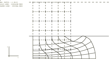
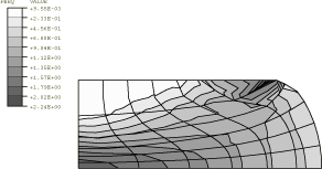
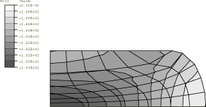
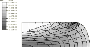
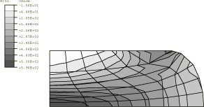
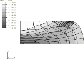
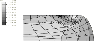
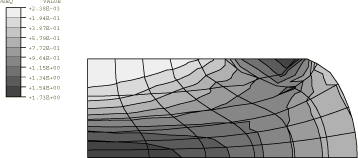
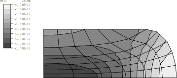
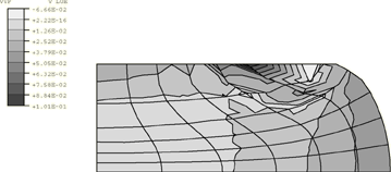
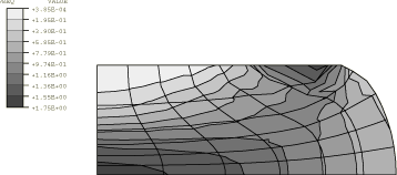
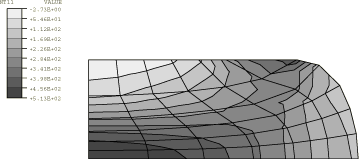
The results of the Abaqus/Standard simulations are discussed first, beginning with the results for the viscoplastic fully dense material. The results of the slow upsetting are illustrated in Figure 2 to Figure 4. The results for the fast upsetting coupled temperature-displacement analysis are illustrated in Figure 5 to Figure 7; those for the adiabatic static stress analysis are shown in Figure 8 and Figure 9. Figure 2 and Figure 5 show the configuration that is predicted at 60% upsetting. The configuration for the adiabatic analysis is not shown since it is almost identical to the fast upsetting coupled case. Both the slow and the fast upsetting cases show the folding of the top outside surface of the billet onto the die, as well as the severe straining of the middle of the specimen. The second figure in each series (Figure 3 for the slow case, Figure 6 for the fast case, and Figure 8 for the adiabatic case) shows the equivalent plastic strain in the billet. Peak strains of around 180% occur in the center of the specimen. The third figure in each series (Figure 4 for the slow case, Figure 7 for the fast case, and Figure 9 for the adiabatic case) shows the temperature distributions, which are noticeably different between the slow and fast upsetting cases. In the slow case there is time for the heat to diffuse (the 60% upsetting takes place in 100 sec, on a specimen where a typical length is 10 mm), so the temperature distribution at 100 sec is quite uniform, varying only between 180°C and 185°C through the billet. In contrast, the fast upsetting occurs too quickly for the heat to diffuse. In this case the middle of the top surface of the specimen remains at 0°C at the end of the event, while the center of the specimen heats up to almost 600°C. There is no significant difference in temperatures between the fast coupled case and the adiabatic case. In the outer top section of the billet there are differences that are a result of the severe distortion of the elements in that region and the lack of dissipation of generated heat. The temperature in the rest of the billet compares well. This example illustrates the advantage of an adiabatic analysis, since a good representation of the results is obtained in about 60% of the computer time required for the fully coupled analysis.
The results of the slow and fast upsetting of the billet modeled with the porous metal plasticity model are shown in Figure 10 to Figure 15. The deformed configuration is identical to that of Figure 2 and Figure 5. The extent of growth/closure of the voids in the specimen at the end of the analysis is shown in Figure 10 and Figure 13. The porous material is almost fully compacted near the center of the billet because of the compressive nature of the stress field in that region; on the other hand, the corner element is folded up and stretched out near the outer top portion of the billet, increasing the void volume fraction to almost 0.1 (or 10%) and indicating that tearing of the material is likely. The equivalent plastic strain is shown in Figure 11 (slow upsetting) and Figure 14 (fast upsetting) for the porous material; Figure 12 and Figure 15 show the temperature distribution for the slow and the fast upsetting of the porous metal. The porous metal needs less external work to achieve the same deformation compared to a fully dense metal. Consequently, there is less plastic work being dissipated as heat; hence, the temperature increase is not as much as that of fully dense metal. This effect is more pronounced in the fast upsetting problem, where the specimen heats up to only 510°C, compared to about 600°C for fully dense metal.
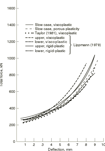
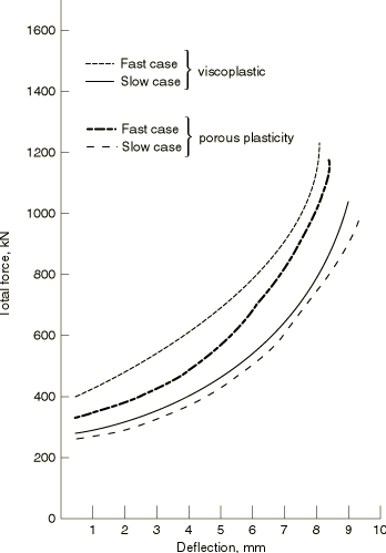
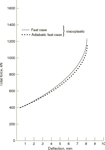
Figure 16 to Figure 18 show predictions of total upsetting force versus displacement of the die. In Figure 16 the slow upsetting viscoplastic and porous plasticity results are compared with several elastic-plastic and rigid-plastic results that were collected by Lippmann (1979) and slow viscoplastic results obtained by Taylor (1981). There is general agreement between all the rate-independent results, and these correspond to the slow viscoplastic results of the present example and of those found by Taylor (1981). In Figure 17 rate dependence of the yield stress is investigated. The fast viscoplastic and porous plasticity results show significantly higher force values throughout the event than the slow results. This effect can be estimated easily. A nominal strain rate of 6 sec is maintained throughout the event. With the viscoplastic model that is used, this effect increases the yield stress by 68%. This factor is very close to the load amplification factor that appears in Figure 17. Figure 18 shows that the force versus displacement prediction of the fast viscoplastic adiabatic analysis agrees well with the fully coupled results.
Two cases using an element-based rigid surface to model the die are also considered in Abaqus/Standard. To define the element-based rigid surface, the elements are assigned to rigid bodies using an isothermal rigid body constraint. The results agree very well with the case when the analytical rigid surface is used.
The automatic load incrementation results suggest that overall nominal strain increments of about 2% per increment were obtained, which is slightly better than what was anticipated in the initial time increment suggestion. These values are typical for problems of this class and are useful guidelines for estimating the computational effort required for such cases.
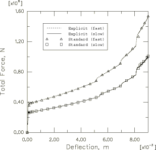
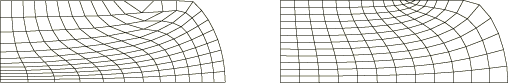
The results obtained with Abaqus/Explicit compare well with those obtained with Abaqus/Standard, as illustrated in Figure 19, which compares the results obtained with Abaqus/Explicit (without adaptive meshing) for the total upsetting force versus the displacement of the die against the same results obtained with Abaqus/Standard. The agreement between the two solutions is excellent. Similar agreement is obtained with the results obtained from the Abaqus/Explicit simulation using adaptive meshing. The mesh distortion is significantly reduced in this case, as illustrated in Figure 20.
![]()
Input files
Abaqus/Standard input files
- cylbillet_cax4t_slow_dense.inp
Slow upsetting case with 144 CAX4T elements, using the fully dense material.
- cylbillet_cax4t_fast_dense.inp
Fast upsetting case with 144 CAX4T elements, using the fully dense material.
- cylbillet_cax4rt_slow_dense.inp
Slow upsetting case with 144 CAX4RT elements, using the fully dense material.
- cylbillet_cax4rt_fast_dense.inp
Fast upsetting case with 144 CAX4RT elements, using the fully dense material.
- cylbillet_cax8rt_slow_dense.inp
Slow upsetting case with CAX8RT elements, using the fully dense material.
- cylbillet_cax8rt_rb_s_dense.inp
Slow upsetting case with CAX8RT elements, using the fully dense material and an element-based rigid surface for the die.
- cylbillet_cax8rt_fast_dense.inp
Fast upsetting case with CAX8RT elements, using the fully dense material.
- cylbillet_cax8rt_slow_por.inp
Slow upsetting case with CAX8RT elements, using the porous material.
- cylbillet_cax8rt_fast_por.inp
Fast upsetting case with CAX8RT elements, using the porous material.
- cylbillet_cgax4t_slow_dense.inp
Slow upsetting case with 144 CGAX4T elements, using the fully dense material.
- cylbillet_cgax4t_fast_dense.inp
Fast upsetting case with 144 CGAX4T elements, using the fully dense material.
- cylbillet_cgax4t_rb_f_dense.inp
Fast upsetting case with 144 CGAX4T elements, using the fully dense material and an element-based rigid surface for the die.
- cylbillet_cgax4t_rb_f_dense_surf.inp
Fast upsetting case with 144 CGAX4T elements, using the fully dense material and an element-based rigid surface for the die with surface-to-surface contact.
- cylbillet_cgax8rt_slow_dense.inp
Slow upsetting case with CGAX8RT elements, using the fully dense material.
- cylbillet_cgax8rt_fast_dense.inp
Fast upsetting case with CGAX8RT elements, using the fully dense material.
- cylbillet_c3d10m_adiab_dense.inp
Adiabatic static analysis with fully dense material modeled with C3D10M elements.
- cylbillet_c3d10m_adiab_dense_surf.inp
Adiabatic static analysis with fully dense material modeled with C3D10M elements using surface-to-surface contact.
- cylbillet_c3d10m_adiab_dense_po.inp
POST OUTPUT analysis of cylbillet_c3d10m_adiab_dense.inp.
- cylbillet_cax6m_adiab_dense.inp
Adiabatic static analysis with fully dense material modeled with CAX6M elements.
- cylbillet_cax8r_adiab_dense.inp
Adiabatic static analysis with fully dense material modeled with CAX8R elements.
- cylbillet_postoutput.inp
POST OUTPUT analysis using the fully dense material.
- cylbillet_slow_usr_umat_umatht.inp
Slow upsetting case with the material behavior defined in user subroutines UMAT and UMATHT.
- cylbillet_slow_usr_umat_umatht.f
User subroutines UMAT and UMATHT used in cylbillet_slow_usr_umat_umatht.inp.
Abaqus/Explicit input files
- cylbillet_x_cax4rt_slow.inp
Slow upsetting case with fully dense material modeled with CAX4RT elements and without adaptive meshing; kinematic mechanical contact.
- cylbillet_x_cax4rt_fast.inp
Fast upsetting case with fully dense material modeled with CAX4RT elements and without adaptive meshing; kinematic mechanical contact.
- cylbillet_x_cax4rt_slow_adap.inp
Slow upsetting case with fully dense material modeled with CAX4RT elements and with adaptive meshing; kinematic mechanical contact.
- cylbillet_x_cax4rt_fast_adap.inp
Fast upsetting case with fully dense material modeled with CAX4RT elements and with adaptive meshing; kinematic mechanical contact.
- cylbillet_xp_cax4rt_fast.inp
Fast upsetting case with fully dense material modeled with CAX4RT elements and without adaptive meshing; penalty mechanical contact.
![]()
References
- Metal Forming Plasticity, Springer-Verlag, Berlin, 1979.
- “A Finite Element Analysis for Large Deformation Metal Forming Problems Involving Contact and Friction,” Ph.D. Thesis, U. of Texas at Austin, 1981.
![]()
Figures