Context:
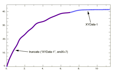
Figure 1 illustrates an X–Y plot that has been truncated at a maximum of 7 by using the function.
Figure 1. X–Y plot produced using the function.
Locate the Operate on XY Data dialog box.
From the main menu bar, select . Click Operate on XY data in the dialog box that appears; then click Continue. The Operate on XY Data dialog box appears.
From the Operators listed, click .
The function appears in the expression window.
From the XY Data choices, click the name of the X–Y data object on which to operate and click Add to Expression. You can choose from all X–Y data objects previously saved within this session (listed alphabetically in the XY Data field).
The X–Y data object name appears within the function parentheses in the expression window.
Specify the X–coordinate values above which or below which data points should be removed from the X–Y data object. To specify a maximum value, position your cursor in the expression window before the second comma, and enter a number for the maximum value. To specify a minimum value, append startX=value to the expression in the expression window.
If desired, customize the truncation order value, which determines whether Abaqus/CAE should create new data points at the truncation boundary or boundaries you specify and, if so, how these new data points should be calculated. Select one of the following:
-
If truncOrder=2 (the default value), Abaqus/CAE performs a piecewise, linear fit on the data to determine a new data point at each boundary and includes the new point or points in the new X–Y data object.
-
If truncOrder=3, Abaqus/CAE performs a spline interpolation on the data to determine a new data point at each boundary and includes the new point or points in the new X–Y data object.
-
If truncOrder=1, Abaqus/CAE does not create any new points at the boundary values.
If desired, customize the truncation tolerance value. If you elect to include interpolated values at the truncation boundaries, the truncation tolerance value overrides the creation of these new data points if Abaqus/CAE finds existing data points that are already very close to the boundaries. By default, the truncation tolerance (truncTol) is 0.005, or one half of one percent of the average distance in the X-direction between adjacent data points in the X–Y data object. If Abaqus/CAE finds an existing data point closer to the truncation boundary than the truncation tolerance value, it does not create a new interpolated data point at that boundary.
To continue to build your expression, position the cursor in the expression window and type in or select the functions, operators, and X–Y data you want to include.
To evaluate and display your expression, click Plot Expression.
To save your new X–Y data object, click Save As and then provide a name in the dialog box that appears.
Saving your data object makes it available for future operations within this session and for inclusion in X–Y plots containing multiple data objects.
When you are finished, click Cancel to close the dialog box.