Interpolating an X–Y data object

Use the interpolate function to operate on a previously saved X–Y data object (a collection of ordered pairs) to produce a new X–Y data object. Interpolating an X–Y data object with nonuniform data produces an X–Y data object with new, interpolated Y-coordinate values occurring at regular increments on the X-axis. By default, the data are interpolated at increments equal to the smallest X-increment in the source data.

Related Topics
Using X–Y data operations

Context:

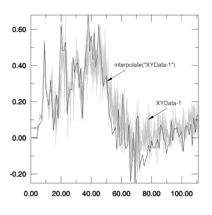
Figure 1 shows an example of an X–Y plot produced using the interpolate function, superimposed over the raw data.

Figure 1. X–Y plot produced using the interpolate function.

The name of the X–Y data object is the only required argument for the interpolate function. A description of the optional arguments follows:

  • The X-axis increment between interpolated data points (xIncrement). If you do not specify a value for this argument or if you specify a non-positive value, Abaqus/CAE uses the minimum X-increment of the raw data set.

  • A symbolic constant that specifies the interpolation scheme (interpolation). Valid values for this argument are QUADRATIC, specifying a Lagrange second-order interpolation scheme; CUBIC_SPLINE, specifying a cubic spline interpolation scheme; and LINEAR, specifying a linear interpolation scheme. The default value is QUADRATIC.

  • The slope of the raw data curve leading up to the first data point (startslope). This argument's default value is 0.0 (for a level slope), and it is used only when interpolation=CUBIC_SPLINE.

  • The slope of the raw data curve continuing past the final data point (endslope). This argument's default value is 0.0 (for a level slope), and it is used only when interpolation=CUBIC_SPLINE.

  1. Locate the Operate on XY Data dialog box.

    From the main menu bar, select ToolsXY DataCreate. Click Operate on XY data in the dialog box that appears; then click Continue. The Operate on XY Data dialog box appears.

  2. From the Operators listed, click interpolate(X).

    The interpolate function appears in the expression window.

  3. From the XY Data choices, click the name of the X–Y data object on which to operate and click Add to Expression. You can choose from all X–Y data objects previously saved within this session (listed alphabetically in the XY Data field).

    The X–Y data object name appears within the interpolate function parentheses in the expression window.

  4. To continue to build your expression, position the cursor in the expression window and type in or select the functions, operators, and X–Y data you want to include.

  5. To evaluate and display your expression, click Plot Expression.

  6. To save your new X–Y data object, click Save As and then provide a name in the dialog box that appears.

    Saving your data object makes it available for future operations within this session and for inclusion in X–Y plots containing multiple data objects.

  7. When you are finished, click Cancel to close the dialog box.