Context:
Figure 1 and Figure 2 show examples of X–Y plots produced using the function using each curve fitting algorithm.
Figure 1. X–Y plot produced using the function with the linear least squares option selected.
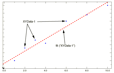
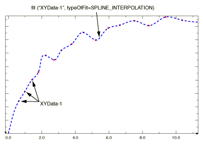
Figure 2. X–Y plot produced using the function with the spline interpolation option selected.
Locate the Operate on XY Data dialog box.
From the main menu bar, select . Click Operate on XY data in the dialog box that appears; then click Continue. The Operate on XY Data dialog box appears.
From the Operators listed, click .
The function appears in the expression window with the linear least squares fit option selected by default.
From the XY Data choices, click the name of the X–Y data object on which to operate and click Add to Expression. You can choose from all X–Y data objects previously saved within this session (listed alphabetically in the XY Data field).
The X–Y data object name appears within the function parentheses in the expression window.
To continue to build your expression, position the cursor in the expression window and type in or select the functions, operators, and X–Y data you want to include. You can customize the function itself by including the following changes to its options:
-
If you want to perform a spline interpolation, set the typeOfFit option to SPLINE_INTERPOLATION.
-
If you want to specify a custom number of points to be created for the new X–Y data object, append numFitPoints=number. By default, Abaqus/CAE uses 2 points to define a linear least squares fit and 100 points to define a spline interpolation.
To evaluate and display your expression, click Plot Expression.
To save your new X–Y data object, click Save As and then provide a name in the dialog box that appears.
Saving your data object makes it available for future operations within this session and for inclusion in X–Y plots containing multiple data objects.
When you are finished, click Cancel to close the dialog box.