Understanding ply stack plots | ||
| ||
You can customize the appearance of a ply stack plot. For example, the image can show the sequence of plies, the orientation of the fibers in each ply, the material in each ply, the relative thickness of the ply, and the location of the reference surface. Figure 1 illustrates a ply stack plot.
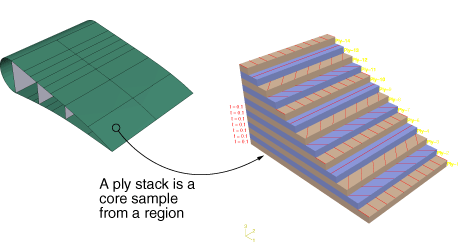
The staircase appearance has no corresponding physical meaning; it is just a mechanism that allows you to view all of the plies in a region. For example, the plies are not ending at each stair.
The triad in a ply stack plot represents the element orientation system, and it shows the shell normal or stacking direction (the 3-direction) and the 1- and 2-directions for the plies. The fibers are always drawn in the 1–2 plane at an angle with respect to the 1-direction. In solid composite layups the fibers in a ply do not always run parallel to the 1–2 plane (e.g., if the 3-direction of the ply orientation and the element stacking direction are not aligned). In this situation the fibers in the ply stack plot are not a true depiction of the fibers in the composite, but rather a graphical representation of the rotation angles in the composite section or layup definition: the angle drawn in the ply stack plot is the rotation angle specified in the ply table measured about the element stacking direction axis. For more information, see Understanding composite layups and orientations.
Ply stack plots do not draw fibers for ply orientations that are based on a user-defined coordinate system or a rotation angle distribution. Abaqus/CAE displays an asterisk (for coordinate systems) or a caret (for rotation angle distributions) on such plies to signify that it cannot draw lines in the 1–2 plane that accurately represent the fiber direction for the ply. Similarly, if you use a discrete field distribution to define a ply's thickness, Abaqus/CAE draws the ply in the ply stack plot based on the average thickness of the other uniform plies in the layup and displays the discrete field name next to the plot (if thickness labels are turned on).
It is important to know the position of the reference surface when you are modeling a composite with conventional shell elements. The mesh will be positioned on the reference surface, and contact is defined relative to the reference surface. The ply stack plot allows you to view the reference surface relative to other plies in the composite, as shown in Figure 2.

You can display a ply stack plot in the Property module after you have created a composite layup or assigned a composite section to a region. You can also display a ply stack plot in the Visualization module after you have analyzed a model with a composite layup or a composite section. For more information, see Defining composite layups and Creating composite shell sections.
To produce a ply stack plot, select
from the main menu bar and select Ply stack plot from the
dialog box that appears. After you have displayed a ply stack plot, you can
customize its appearance by clicking the button from the prompt area or by clicking the
 tool in the toolbox (in
the Visualization module).
For detailed instructions on customizing a ply stack plot, see
Customizing ply stack plots.
tool in the toolbox (in
the Visualization module).
For detailed instructions on customizing a ply stack plot, see
Customizing ply stack plots.