About co-simulation | ||
| ||
Abaqus provides built-in procedures to solve multiphysics simulations as described in Multiphysics analyses. For multiphysics problems for which Abaqus does not provide a built-in solution procedure or where the solution procedure is limited in functionality, you can use the co-simulation technique to couple Abaqus with a third-party analysis program; for example, fluid-structure interaction (FSI) simulation in conjunction with computational fluid dynamics (CFD) analysis programs.
Co-simulation between Abaqus/Standard and Abaqus/Explicit illustrates a multiple domain analysis approach, where each Abaqus analysis operates on a complementary section of the model domain where it is expected to provide the more computationally efficient solution. For example, Abaqus/Standard provides a more efficient solution for light and stiff components, while Abaqus/Explicit is more efficient for solving complex contact interactions.
Features of the Abaqus co-simulation technique
The Abaqus co-simulation technique:
-
can be used to solve complex fluid-structure interactions by coupling Abaqus with CFD analysis programs;
-
can be used to solve problems involving electromagnetic-thermal or electromagnetic-mechanical interactions by coupling Abaqus with an electromagnetic analysis program, including electromagnetic analysis procedures in Abaqus/Standard;
-
can be used for multiphysics simulations by coupling Abaqus with third-party analysis programs;
-
can be used to solve complex multidomain analyses more effectively by coupling Abaqus/Standard to Abaqus/Explicit;
-
can be used to solve structural-to-logical simulations by coupling Abaqus/Standard or Abaqus/Explicit with Dymola;
-
can be used to couple Abaqus with in-house codes using the SIMULIA Co-Simulation Engine;
-
is intended for advanced users with in-depth knowledge of Abaqus and the third-party analysis program;
-
allows for both unidirectional and bidirectional transfer of data;
-
can be used with Abaqus models having linear or nonlinear structural response; and
-
supports steady-state, transient, and, for electromagnetic procedures, time-harmonic simulations.
![]()
Interaction between domains modeled with different analysis programs
In a co-simulation the interaction between the domains is through a common physical interface region over which data are exchanged in a synchronized manner between Abaqus and the coupled analysis program.
One domain may affect the response of another domain through one or more of the following:
-
the constitutive behavior, such as the yield stress defined as a function of temperature or stress defined as a function of other solution fields, such as thermal strains or the piezoelectric effect;
-
surface tractions/fluxes, such as a fluid exerting pressure on a structure;
-
body forces/fluxes, such as heat generation due to flow of current in a coupled thermal-electrical simulation;
-
contact forces, such as the forces due to contact between a vehicle and an occupant/pedestrian modeled as separate domains;
-
kinematics, such as fluid in contact with a compliant structure where the interface motion affects the fluid flow; and
-
discrete coupling, such as sensor and actuation information.
Coupling Abaqus using the SIMULIA Co-Simulation Engine
The SIMULIA Co-Simulation Engine provides coupling between Abaqus analyses or between Abaqus and third-party analysis programs. This coupling method is used for fluid-structure, conjugate heat transfer, electromagnetic-structural, electromagnetic-thermal, and structural-logical simulations, and when coupling Abaqus/Standard to Abaqus/Explicit for interaction between implicit dynamic and explicit dynamic domains.
Fluid-structure interaction
You can solve complex fluid-structure interaction (FSI) problems by coupling Abaqus/Standard or Abaqus/Explicit to a computational fluid dynamics (CFD) analysis program. Abaqus/Standard and Abaqus/Explicit solve the structural domain, and the CFD analysis program solves the fluid domain. Abaqus/Standard and Abaqus/Explicit can be coupled with several third-party CFD analysis programs.
For a complete list of qualified partner products, see the http://www.3ds.com/support/certified-hardware/simulia-system-information/compatibility/co-simulation/ page at www.3ds.com/simulia.
Conjugate heat transfer
You can solve conjugate heat transfer problems involving fluids and structures by coupling Abaqus/Standard to a computational fluid dynamics (CFD) analysis program. Abaqus/Standard models heat transfer within the structure (see Uncoupled heat transfer analysis and Fully coupled thermal-stress analysis), and the CFD analysis program solves the energy equation for the fluid flow surrounding the structure. Abaqus/Standard can be coupled with several third-party CFD analysis programs.
For a complete list of qualified partner products, see the http://www.3ds.com/support/certified-hardware/simulia-system-information/compatibility/co-simulation/ page at www.3ds.com/simulia.
Electromagnetic-thermal or electromagnetic-mechanical coupling
Applications such as induction heating require interaction between electromagnetic and thermal fields. You can solve this class of problems by coupling two Abaqus/Standard analyses, where one analysis solves for the fields in the electromagnetic domain, while the other solves for the fields in the thermal domain. Abaqus/Standard can be coupled with itself, as well as with several third-party electromagnetic analysis programs.
For detailed information on coupling Abaqus/Standard to Abaqus/Standard, see Preparing an Abaqus analysis for co-simulation and Electromagnetic-to-structural and electromagnetic-to-thermal co-simulation. For a complete list of qualified partner products, see the http://www.3ds.com/support/certified-hardware/simulia-system-information/compatibility/co-simulation/ page at www.3ds.com/simulia.
System-level modeling via logical-physical interaction
System-level modeling refers to modeling of systems that may include both physical (structural, thermal, acoustics, etc.) and logical components. The distinction between the two modeling abstractions is as follows:
-
Logical modeling refers to a large class of modeling abstractions often encountered in the engineering practice. Generally speaking, you can designate a part of a system as using a logical modeling abstraction when most (if not all) of the geometry of the part is removed. Examples include electronic control modules, electric motors, and pneumatic or hydraulic subsystems, which in many cases can be modeled from a functional perspective without attempting to model the flow of electrons, the variation of magnetic fluxes, or the air/fluid type of flow in ducts and pipes. Dymola offers a variety of logical modeling options.
-
Physical modeling is the complementary modeling abstraction to logical modeling. Abaqus uses a physical modeling abstraction most of the time; as elements deform, they know precisely about their geometry, thus trying to mimic the real world at a fine-grain level.
In many engineering systems the interaction between logical and physical components is paramount, and you cannot fully analyze one without the other. Co-simulation using Abaqus and Dymola provides the capability to analyze this type of system.
Consider the example of a rolling mill: the incoming slab, which may not have a constant thickness, can be modeled in Abaqus as being deformed by the rolling cylinders. Because of the nonconstant incoming thickness, a pressure that adapts as a function of deformation needs to be exerted on the cylinders to compensate such that the exit thickness is as constant as possible. Abaqus sensors can export the information about the mechanical status of the system to Dymola, which in turn could use this information to model the necessary compensators to calculate the needed actuation load at any given time. Abaqus can import the actuation load and apply it to the cylinders.
For detailed information on coupling Abaqus/Standard to Dymola, see Structural-to-logical co-simulation. For a complete list of qualified partner products, see the http://www.3ds.com/support/certified-hardware/simulia-system-information/compatibility/co-simulation/ page at www.3ds.com/simulia.
Interaction between an implicit transient analysis and an explicit dynamics analysis
In certain cases you can realize significant computational cost savings by partitioning a model and combining the Abaqus/Standard and Abaqus/Explicit solutions, such as
-
when the simulation is principally a candidate for Abaqus/Explicit, but where certain parts of the model can be idealized using substructures in Abaqus/Standard, or
-
when the simulation is principally a candidate for Abaqus/Standard, but where complex contact conditions would be handled more effectively by Abaqus/Explicit.
For an example of Abaqus/Standard to Abaqus/Explicit co-simulation, refer to Dynamic impact of a scooter with a bump. For detailed information on coupling Abaqus/Standard and Abaqus/Explicit, see Preparing an Abaqus analysis for co-simulation and Structural-to-structural co-simulation.
Coupling using the MpCCI interface
MpCCI, the multiphysics code coupling interface developed and distributed by the Fraunhofer-Institute for Algorithms and Scientific Computing (SCAI), provides an open system approach for general multidisciplinary simulations between Abaqus and any third-party analysis program that supports MpCCI. MpCCI provides a scalable communication infrastructure and mapping algorithms for multiple physics domains. In a co-simulation using MpCCI, Abaqus communicates in real time with the MpCCI coupling server to exchange fields with the third-party analysis program while each analysis advances its simulation time.
Coupling through MpCCI may occur between Abaqus and any third-party analysis program that supports the MpCCI interface. This includes in-house codes that have the MpCCI adapter embedded. SIMULIA actively supports and qualifies a link between Abaqus and FLUENT for fluid-structure interaction. For further information on coupling using the MpCCI interface, contact http://www.mpcci.de.
Additional applications
There are many other applications for which co-simulation can be employed with partner products. For example, vehicle ride comfort and durability simulation using FTire from http://www.cosin.eu. For a complete list of qualified partner products, see the http://www.3ds.com/support/certified-hardware/simulia-system-information/compatibility/co-simulation/ page at www.3ds.com/simulia.
![]()
Strength of physics coupling
You will typically apply co-simulation techniques to problems where the most complex physics occurs within domains that are handled exclusively within an analysis program (e.g., Abaqus or a CFD analysis program). Due to the comparative numerical simplicity of the numerical techniques applied at the co-simulation interface, the physics controlling the interaction at the interface of the separate analysis domains (the strength of the physics coupling) must be relatively weak for the co-simulation technique to be applied effectively.
Coupling to third-party analysis programs
Analysis domains are coupled in a staggered approach either using a globally explicit manner or an implicit iterative manner; that is, the equations for each domain are solved separately, and loads and boundary conditions are exchanged at the common interface.
In cases where the coupling is sufficiently weak, the coupling may be required only in one direction (such as when an electromagnetic force field contributes to the structural response, but a reverse coupling provides no significant impact on the electromagnetic field).
In an explicit staggered approach, such as the Gauss-Seidel coupling scheme, fields are exchanged only once per coupling step. This coupling strategy is applicable to problems that exhibit weak to moderate physics coupling (for example, aeroelasticity problems where you have air interacting with a relatively stiff structure). The explicit staggered approach requires a small coupling step size.
In an implicit iterative approach, the fields are exchanged multiple times per coupling step until an overall equilibrium is achieved prior to advancing to the next coupling step. Implicit coupling is computationally more expensive per coupling step and generally can be employed to problems exhibiting moderate to strong physics coupling. In general, a larger coupling step size can be employed than for explicit schemes.
Figure 1 illustrates the coupling strength with an analogy in the frequency domain. Consider a lumped parameter dynamic system with a coupling impedance directly related to a response frequency . In a staggered solution approach each domain is solved by temporarily ignoring the coupling terms represented by the gray spring and dashpot in Figure 1.
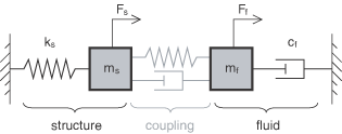
When the response frequency and coupling impedance are low, a staggered approach will likely provide adequate solution accuracy and performance. However, when the response frequency is high, such that the coupling impedance is relatively large compared to the structure or fluid, you may encounter solution stability issues with the staggered approach.
Coupling in Abaqus/Standard to Abaqus/Explicit co-simulation
The strength of the physics coupling can generally be greater in the coupling of Abaqus/Standard to Abaqus/Explicit using the co-simulation technique. Through communication of “right-hand-side” and “left-hand-side” terms, Abaqus/Standard to Abaqus/Explicit co-simulation provides a robust interface solution across a wide range of problem parameters. In many cases you can choose to have Abaqus/Standard and Abaqus/Explicit each advance their solutions according to their own automatic time incrementation scheme without adversely affecting the interface solution stability.
![]()
References
For the latest support information and tips on running FSI simulations and crash safety simulations, see the Dassault Systèmes Knowledge Base at http://www.3ds.com/support/knowledge-base.