Stress rates | ||||||
|
| |||||
ProductsAbaqus/StandardAbaqus/Explicit
Many of the materials we wish to model with Abaqus are history dependent, and it is common for the constitutive equations to appear in rate form. In Stress measures it was suggested that an appropriate stress measure for stress-sensitive materials (such as yielding materials) is the Kirchhoff stress. We, therefore, need to define the rate of Kirchhoff stress for use in the constitutive equations. This definition is not simply the material time rate of Kirchhoff stress, because the Kirchhoff stress components are associated with spatial directions in the current configuration (recall that the Kirchhoff stress is , where J is the volume change from the reference configuration and is the Cauchy stress, defined by , where and are vectors in the current configuration).
To illustrate the issue, consider a uniaxial tension specimen under constant axial force P, lying along the x-axis at time and rotated—with the axial force held constant—to lie along the y-axis at time (see Figure 1).
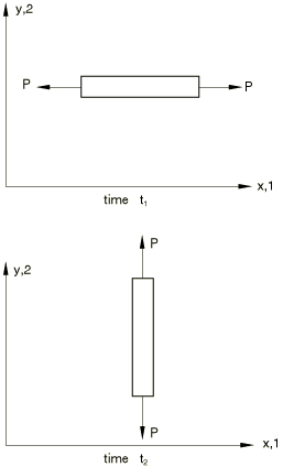
Write the stress components on the global rectangular Cartesian basis. At time , , and all other , while at time , , and all other . Obviously during , and , but equally clearly this rate of change of stress has nothing to do with the constitutive response of the material making up the bar. (A materially based stress, such as the second Piola-Kirchhoff stress, would stay constant during the above rotation, because its components are associated with a material basis.) The problem, then, is that the components of or are associated with current directions in space and, therefore, and will be nonzero if there is pure rigid body rotation, even though from a constitutive point of view the material is unchanged. Thus, we must divide the increment of or into two parts—one attributable to rigid body motion only and a remainder that is then, presumably, associated with the rate form of the stress-strain law.
We can derive a simple result for this purpose for any matrix whose components are associated with spatial directions. At some time t imagine attaching to a material point a set of base vectors, , These vectors cannot stretch but are defined to spin with the same spin as the material. Recall that the spatial gradient of the material particle velocity at a point, , was decomposed into a rate of deformation and a spin,
One of the concepts of the motion of the base vectors in Abaqus is that
Another concept of the motion of the base vectors used in Abaqus is
where . Here is the rigid body rotation in the polar decomposition of the deformation gradient . The differences between these two concepts are significant only if finite rotation of a material point is accompanied by finite shear.
Now consider any matrix based on the current configuration: we can write it in terms of its components in the directions:
Taking the time derivative then gives
The second and third terms are the rate of caused by the rigid body spin, so the first term is that part of caused by other effects (in the case of stress, the rate associated with the constitutive response), called the corotational rate of . From the definitions of as rigid base vectors that can be considered to spin with either or , we can write two corotational rates of as
and
where and are called the Jaumann and Green-Naghdi rates, respectively.
We, thus, have the total rate of any matrix associated with spatial directions in the current configuration as the sum of the corotational rate of the matrix and a rate caused purely by the local spin or rigid body rotation. For example, the Jaumann rate of change of Kirchhoff stress can be written as
We are assuming that the constitutive theory will define , the corotational stress rate per reference volume, in terms of the rate of deformation and past history, so this equation provides a convenient link between that material model and the overall change in “true” (Cauchy) stress (which is the stress measure defined directly from the equilibrium equations). In Mechanical Constitutive Theories where the constitutive models in Abaqus are discussed, “stress rate” per reference volume will mean , the corotational rate of Kirchhoff stress, which is the stress measure work conjugate to the rate of deformation.
Stress rates used in Abaqus
The objective stress rates used in Abaqus are summarized in Table 1. Objective rates are relevant only for rate form constitutive equations (e.g., elastoplasticity). For hyperelastic materials a total formulation is used; hence, the concept of an objective rate is not relevant for the constitutive law. However, when material orientations are defined, the objective rate governs the evolution of the orientations and the output will be affected.
| Solver | Element Type | Constitutive Model | Objective Rate |
|---|---|---|---|
| Abaqus/Standard | Solid (Continuum) | All built-in and user-defined materials | Jaumann |
| Structural (Shells, Membranes, Beams, Trusses) | All built-in and user-defined materials | Green-Naghdi | |
| Abaqus/Explicit | Solid (Continuum) | All except hyperelastic, viscoelastic, brittle cracking, and VUMAT | Jaumann |
| Solid (Continuum) | Hyperelastic, viscoelastic, brittle cracking, and VUMAT | Green-Naghdi | |
| Structural (Shells, Membranes, Beams, Trusses) | All built-in and user-defined materials | Green-Naghdi |