Line spring elements | ||||||
|
| |||||
ProductsAbaqus/Standard
The “line spring” is a series of one-dimensional finite elements placed along the part-through flaw, which allows local flexibility of one side of the flaw with respect to the other (points A and B in Figure 1). This local flexibility is calculated from existing solutions for single edge notch specimens in plane strain (Figure 2). The approach is computationally inexpensive compared to fully three-dimensional models of the vicinity of the flaw; it is also approximate because of the use of two-dimensional solutions embedded in the shell model. Practical experience with the method on typical geometries has shown that, for several important geometries, the method provides acceptable accuracy.
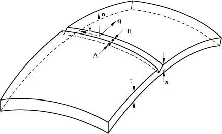
This section discusses the geometric and kinematic basis of the elements as well as the equilibrium statement and the development of the local solutions that define the constitutive relationships. The constitutive relations are expressed in terms of the forces and moments carried across the crack and the relative displacements and rotations of points on opposite sides of the crack (A and B in Figure 1), and are derived from local solutions to single edge cracked plane strain specimens. Elastic and fully plastic (limit analysis) solutions are used to construct an approximate elastic-plastic model.
At each point along the flaw a local orthonormal basis system is defined , with the tangent to the shell along the flaw, the normal to the shell, and defined as
We use the shell normal, , to determine the side of the shell on which the flaw occurs; flaws that open on the positive side are given positive flaw depths to indicate this, and those on the negative side are given negative flaw depths. The relative motion between two points—A and B in Figure 1—on opposite sides of the flaw but otherwise at the same place, then defines a set of six generalized strains as follows. Side B of the element contains nodes 1, 2, 3; and for LS6 elements side A contains nodes 4, 5, and 6.
Mode I:
| opening displacement | |
| opening rotation |
Mode II: through-thickness shear is defined by the relative displacement,
Mode III: antiplane shear is defined by the relative displacement,
and by the relative rotation,
The relative rotation plays no role in the deformation.
These relative motions form the kinematic basis of the element.
Since the line spring elements are written for geometrically linear analysis only, the first variations of these relative motions are identical to the above definitions, with the total values replaced by their variations.
Virtual work contribution
The virtual work contribution of the element is defined as
where , etc., are forces and moments per unit length of flaw that are conjugate to the corresponding relative displacement and rotation values. In the above expression the integration is taken along the entire flaw.
![]()
Interpolation
The elements use quadratic interpolation of displacement and rotation components along the crack, so they are compatible with the second-order shell elements (S8R, S8R5, S9R5, STRI65).
Two line spring elements are provided—LS6 is a general element for use with arbitrary flaws in a shell, while LS3S is provided for Mode I use in cases when the crack lies on a plane of symmetry and the deformation will be symmetric about the same plane, so that only one-half of the geometry must be modeled.
![]()
Elasticity
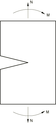
The Mode I line spring compliance is based on a single edge notched specimen subject to far-field tension and bending, as shown in Figure 2. This compliance is
where the matrix can be obtained from the energy compliance calibrations of Rice (1972). The inverse of provides the Mode I stiffness per unit length of flaw, relating and to and . Similar results in Mode II and Mode III complete the elastic stiffness.
Stress intensity factors are calculated as
where approximate expressions for and are given by Tada et al. (1973), and similar expressions apply for Mode III and (without ) for Mode II. The J-integral is then calculated by combining these stress intensities as
where
E is Young's modulus and is Poisson's ratio.
![]()
Plasticity
The elastic-plastic line spring model in Abaqus is based on Mode I response only, since no theory is available for an elastic-plastic line spring model in mixed mode loading. For convenience we define a generalized “strain” vector as
and conjugate generalized “forces” as
The formalism of a simple associated flow, isotropic hardening plasticity model is used as follows. The generalized strain rate is decomposed into elastic and plastic response as
and the Mode I elasticity relationship described above is used to define the generalized stresses:
The plastic strain rate is defined to be normal to a yield surface, :
where is the yield function, whose definition is discussed in detail below, and is a scalar hardening parameter used to provide isotropic hardening. The hardening is calculated from the basic stress-strain data for the material by a work equivalency argument. The plastic work per unit length of flaw is
and is also given by
where is the uniaxial stress-strain behavior of the material and z and y measure position through the thickness and along the length of the single edge notch specimen. We approximate this second expression by
where is a representative value of the yield stress (at an equivalent plastic strain of ); t is the shell thickness; a is the flaw depth; and f is a constant, introduced to provide a matching to numerical results for the specimen. Parks and White (1982) suggest choosing , and this value is used in Abaqus.
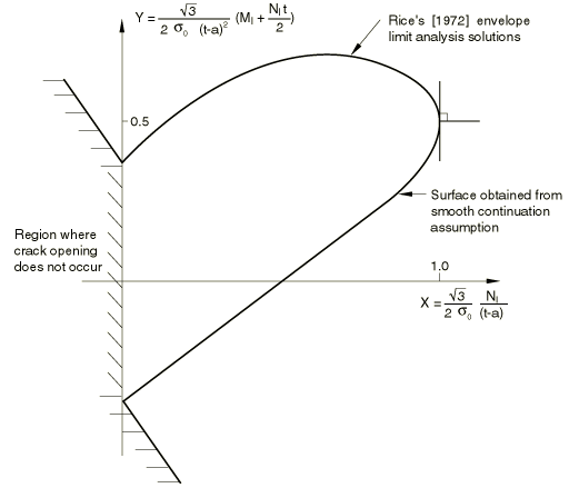
The yield surface is defined with respect to the generalized stress variables and as follows. Following Rice (1972), we define
and
Then for the yield function, , is taken as an envelope to limit analysis results, as proposed by Rice:
Otherwise, we use
with
This surface is chosen to blend continuously with at and as a reasonable estimate of the behavior for . It is, otherwise, arbitrary. Rice (1972) points out that at , the yield surface will have a vertex. The smooth surface used in Abaqus has been adopted for numerical reasons. This smoothness restricts the possible flow behavior at , but we assume that this is not a critical issue.
These surfaces are shown in Figure 3. The figure also indicates a region where the model is not appropriate (because the crack will close). Warning messages are provided if the generalized stress point enters this region at any integration point.
The plasticity model is integrated by the usual backward Euler method (see Integration of plasticity models for details). Once the plastic strain increments are known, from the kinematics of the slip line field proposed by Rice (1972) for an edge cracked strip, the increment of plastic crack-tip opening is given by
The increment in the plastic part of the J-integral is related to the increment of plastic crack-tip opening by
where m is given by (Parks and White, 1982),
where indicates differentiation with respect to crack depth and indicate differentiation by and , respectively. is either or depending on the state of deformation.
The elastic part of the J-integral is obtained from the generalized stresses by calculating the stress intensity factors as described in the previous section (ignoring plasticity effects). The total J-integral is the sum of the plastic and elastic J-integral contributions. Although the method used for computing the elastic contribution is obviously approximate, it is reasonably accurate if dominates , which is the case once a significant amount of plasticity develops (Parks and White, 1982).