Processing math: 86%

Flexible joint element

The JOINTC elements in Abaqus/Standard provide for flexible joints between two nodes. This section defines the kinematic variables used in JOINTC elements.

The following topics are discussed:

Kinematics
Virtual work

Kinematics

A JOINTC element consists of two nodes, referred to here as nodes 1 and 2. Each node has six degrees of freedom: displacements $u$ and rotations $ϕ$ . A local orientation is defined for the element by the user. In a large-displacement analysis that local system rotates with the first node of the element.

Figure 1. JOINTC geometry.

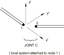
We define the local system by its unit, orthogonal base vectors, $e_{α}$ , for $α = 1, 2, 3$ . Then at any time in the analysis

$e_{α} = C \cdot e_{α}^{0},$

where $C (ϕ^{1})$ is the rotation matrix defined by the rotation at the first node of the element.

The relative displacements in the element are then

$u_{α} = (u^{2} - u^{1}) \cdot e_{α},$

with first variations

$δ u_{α} = (δ u^{2} - δ u^{1}) \cdot e_{α} + δ θ^{1} \cdot e_{α} \times (u^{2} - u^{1}),$

where $δ θ^{1}$ is a linearized rotation field (see Rotation variables), and second variations

$\begin{matrix} d δ u_{α} = & (δ u^{2} - δ u^{1}) \cdot d θ^{1} \times e_{α} + (d u^{2} - d u^{1}) \cdot δ θ^{1} \times e_{α} \\ - d θ^{1} \cdot δ θ^{1} u_{α} + \frac{1}{2} δ θ^{1} \cdot (u^{2} - u^{1}) d θ^{1} \cdot e_{α} + \frac{1}{2} δ θ^{1} \cdot e_{α} d θ^{1} \cdot (u^{2} - u^{1}) . \end{matrix}$

The relative rotation about the local 3-axis is defined as

$ψ_{3} = \frac{1}{2} (e_{1}^{2} - e_{1}^{1}) \cdot (e_{2}^{2} + e_{2}^{1}),$

with $ψ_{1}$ and $ψ_{2}$ defined by cyclic permutation of the local direction indices.

These rotation measures define only relative angular rotations for small relative rotations. They are simple to compute, increase monotonically for relative rotations up to 180°, and are taken as suitable for use in the elements for these reasons.

The first variation of $ψ_{3}$ is

$δ ψ_{3} = \frac{1}{2} (δ θ^{2} \times e_{1}^{2} - δ θ^{1} \times e_{1}^{1}) \cdot (e_{2}^{2} + e_{2}^{1}) + \frac{1}{2} (e_{1}^{2} - e_{1}^{1}) \cdot (δ θ^{2} \times e_{2}^{2} + δ θ^{1} \times e_{2}^{1}),$

and its second variation is

$\begin{matrix} d δ ψ_{3} = & \frac{1}{4} (- 2 d θ^{2} \cdot δ θ^{2} e_{1}^{2} + d θ^{2} \cdot e_{1}^{2} δ θ^{2} + δ θ^{2} \cdot e_{1}^{2} d θ^{2} \\ + 2 d θ^{1} \cdot δ θ^{1} e_{1}^{1} - d θ^{1} \cdot e_{1}^{1} δ θ^{1} - δ θ^{1} \cdot e_{1}^{1} d θ^{1}) \cdot (e_{2}^{2} + e_{2}^{1}) \\ + \frac{1}{4} (e_{1}^{2} - e_{1}^{1}) \cdot (- 2 d θ^{2} \cdot δ θ^{2} e_{2}^{2} + d θ^{2} \cdot e_{2}^{2} δ θ^{2} + δ θ^{2} \cdot e_{2}^{2} d θ^{2} \\ - 2 d θ^{1} \cdot δ θ^{1} e_{2}^{1} + d θ^{1} \cdot e_{2}^{1} δ θ^{1} + δ θ^{1} \cdot e_{2}^{1} d θ^{1}) \\ + \frac{1}{2} (- δ θ^{2} \cdot e_{2}^{2} d θ^{2} \cdot e_{1}^{2} + δ θ^{1} \cdot e_{2}^{1} d θ^{1} \cdot e_{1}^{1} + δ θ^{1} \cdot d θ^{2} (e_{1}^{2} \cdot e_{2}^{1} - e_{1}^{1} \cdot e_{2}^{2})) \\ + \frac{1}{2} (- d θ^{2} \cdot e_{2}^{2} δ θ^{2} \cdot e_{1}^{2} + d θ^{1} \cdot e_{2}^{1} δ θ^{1} \cdot e_{1}^{1} + d θ^{1} \cdot δ θ^{2} (e_{1}^{2} \cdot e_{2}^{1} - e_{1}^{1} \cdot e_{2}^{2})) . \end{matrix}$

The relative translational velocities in the element are taken as

${\dot{u}}_{α} = ({\dot{u}}^{2} - {\dot{u}}^{1}) \cdot e_{α} + {\dot{θ}}^{1} \cdot e_{α} \times (u^{2} - u^{1}),$

and the relative angular velocity about the local 3-axis is taken as

${\dot{ψ}}_{3} = \frac{1}{2} ({\dot{θ}}^{2} \times e_{1}^{2} - {\dot{θ}}^{1} \times e_{1}^{1}) \cdot (e_{2}^{2} + e_{2}^{1}) + \frac{1}{2} (e_{1}^{2} - e_{1}^{1}) \cdot ({\dot{θ}}^{2} \times e_{2}^{2} + {\dot{θ}}^{1} \times e_{2}^{1}) .$

Virtual work

The virtual work contribution of the element is

$δ W = F_{α} δ u_{α} + M_{α} δ ψ_{α} .$

We assume that the behavior of the joint is defined by

$F_{α} = F_{α} (u_{α}, {\dot{u}}_{α}) and M_{α} = M_{α} (ψ_{α}, {\dot{ψ}}_{α}) (no sum on α) .$

The contribution to the operator matrix for the Newton solution is

$d δ W = \sum_{α} δ u_{α} (\frac{\partial F_{α}}{\partial u_{α}} + \frac{\partial F_{α}}{\partial {\dot{u}}_{α}} \frac{\partial \dot{u}}{\partial u}) d u_{α} + δ ψ_{α} (\frac{\partial M_{α}}{\partial ψ_{α}} + \frac{\partial M_{α}}{\partial {\dot{ψ}}_{α}} \frac{\partial \dot{u}}{\partial u}) d ψ_{α} + F_{α} d δ u_{α} + M_{α} d δ ψ_{α},$

where $\partial \dot{u} / \partial u$ is defined by the dynamic time integration operator.