Material properties: hyperelastic model for the rubber | ||
| ||
Context:
The data (shown in Figure 1 and tabulated in Table 1, Table 2, and Table 3) are given in terms of nominal stress and corresponding nominal strain.
Note: Volumetric test data are not required when the material is incompressible (as is the case in this example).

| Stress (Pa) | Strain |
|---|---|
| 0.054E6 | 0.0380 |
| 0.152E6 | 0.1338 |
| 0.254E6 | 0.2210 |
| 0.362E6 | 0.3450 |
| 0.459E6 | 0.4600 |
| 0.583E6 | 0.6242 |
| 0.656E6 | 0.8510 |
| 0.730E6 | 1.4268 |
| Stress (Pa) | Strain |
|---|---|
| 0.089E6 | 0.0200 |
| 0.255E6 | 0.1400 |
| 0.503E6 | 0.4200 |
| 0.958E6 | 1.4900 |
| 1.703E6 | 2.7500 |
| 2.413E6 | 3.4500 |
| Stress (Pa) | Strain |
|---|---|
| 0.055E6 | 0.0690 |
| 0.324E6 | 0.2828 |
| 0.758E6 | 1.3862 |
| 1.269E6 | 3.0345 |
| 1.779E6 | 4.0621 |
When you define a hyperelastic material using experimental data, you also specify the strain energy potential that you want to apply to the data. Abaqus uses the experimental data to calculate the coefficients necessary for the specified strain energy potential. However, it is important to verify that an acceptable correlation exists between the behavior predicted by the material definition and the experimental data.
You can use the material evaluation option available in Abaqus/CAE to simulate one or more standard tests with the experimental data using the strain energy potential that you specify in the material definition.
- To define and evaluate hyperelastic material behavior:
- Create a hyperelastic material named
Rubber. In this example a first-order,
polynomial strain energy function is used to model the rubber material; thus,
select Polynomial from the Strain energy
potential list in the material editor. Enter the test data given
above using the menu items in the material
editor.
To visualize the experimental data, click mouse button 3 on the table for any of the test data and select Create X–Y Data from the menu that appears. You can then plot the data in the Visualization module.
Note: In general, you may be unsure of which strain energy potential to specify. In this case, you could select Unknown from the Strain energy potential list in the material editor. You could then use the Evaluate option to guide your selection by performing standard tests with the experimental data using multiple strain energy potentials.
- In the
Model Tree,
click mouse button 3 on Rubber underneath the
Materials container. Select Evaluate
from the menu that appears to perform the standard unit-element tests
(uniaxial, biaxial, and planar). Specify a minimum strain of
0 and a maximum strain of
1.75 for each test. Evaluate only the
first-order polynomial strain energy function. This form of the hyperelasticity
model is known as the Mooney-Rivlin material model.
When the evaluation is complete, Abaqus/CAE enters the Visualization module. A dialog box appears containing material parameter and stability information. In addition, an X–Y plot that displays a nominal stress–nominal strain curve for the material as well as a plot of the experimental data appears for each test.
- Create a hyperelastic material named
Rubber. In this example a first-order,
polynomial strain energy function is used to model the rubber material; thus,
select Polynomial from the Strain energy
potential list in the material editor. Enter the test data given
above using the menu items in the material
editor.
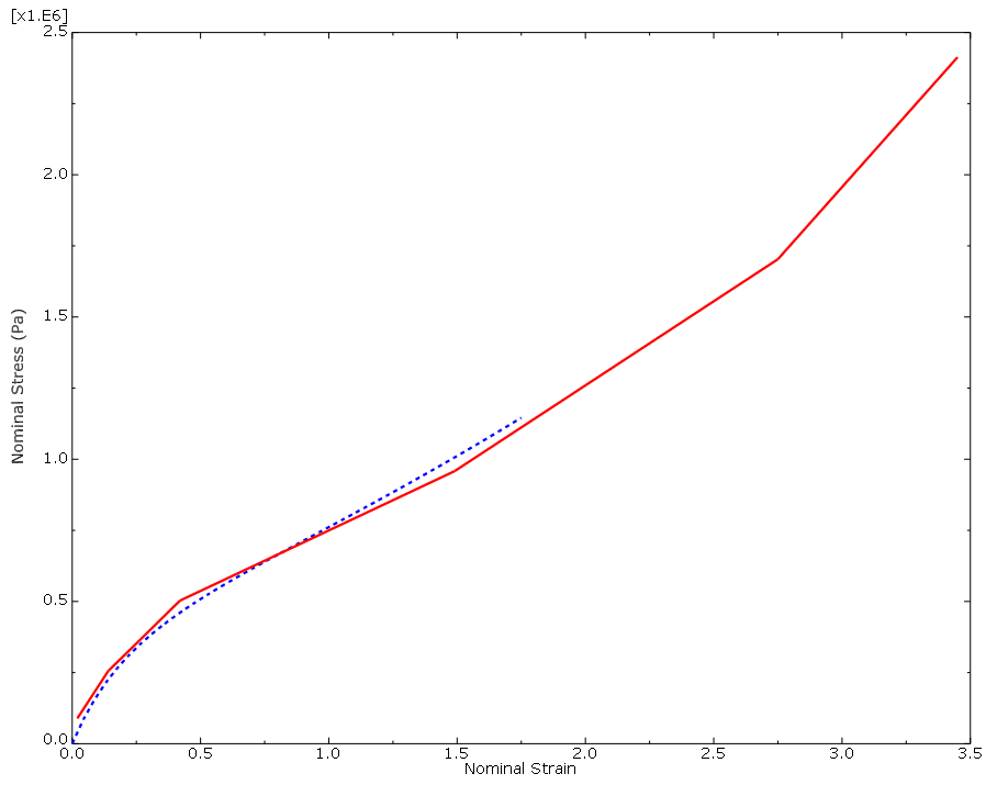
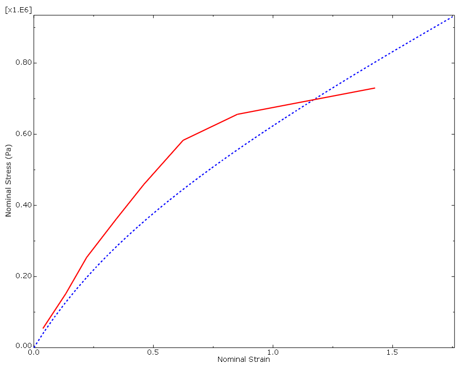
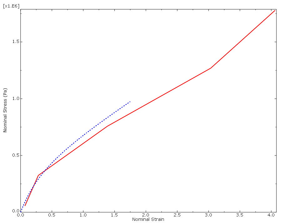
The computational and experimental results for the various types of tests are compared in Figure 2, Figure 3, and Figure 4 (for clarity, some of the computational data points are not shown). The Abaqus/Standard and experimental results for the biaxial tension test match very well. The computational and experimental results for the uniaxial tension and planar tests match well at strains less than 100%. The hyperelastic material model created from these material test data is probably not suitable for use in general simulations where the strains may be larger than 100%. However, the model will be adequate for this simulation if the principal strains remain within the strain magnitudes where the data and the hyperelastic model fit well. If you find that the results are beyond these magnitudes or if you are asked to perform a different simulation, you will have to insist on getting better material data. Otherwise, you will not be able to have much confidence in your results.
- The hyperelastic material parameters
-
In this simulation the material is assumed to be incompressible ( = 0). To achieve this, no volumetric test data were provided. To simulate compressible behavior, you must provide volumetric test data in addition to the other test data.
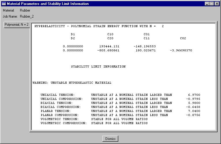
The hyperelastic material coefficients—, , and —that Abaqus calculates from the material test data appear in the Material Parameters and Stability Limit Information dialog box, shown in Figure 5. The material model is stable at all strains with these material test data and this strain energy function.
Figure 5. Material parameters and stability limits for the first-order polynomial strain energy function.
However, if you specified that a second-order (N=2) polynomial strain energy function be used, you would see the warnings shown in Figure 6. If you had only uniaxial test data for this problem, you would find that the Mooney-Rivlin material model Abaqus creates would have unstable material behavior above certain strain magnitudes.
Figure 6. Material parameters and stability limits for the second-order polynomial strain energy function.