Methods of speeding up the analysis | ||
| ||
There are two ways to reduce the cost of the analysis:
-
Artificially increase the punch velocity so that the same forming process occurs in a shorter step time. This method is called load rate scaling.
-
Artificially increase the mass density of the elements so that the stability limit increases, allowing the analysis to take fewer increments. This method is called mass scaling.
Unless the model has rate-dependent materials or damping, these two methods effectively do the same thing.
- Determining acceptable mass scaling
-
Loading rates and Metal forming problems discuss how to determine acceptable scaling of the loading rate or mass to reduce the run time of a quasi-static analysis. The goal is to model the process in the shortest time period in which inertial forces remain insignificant. There are bounds on how much scaling can be used while still obtaining a meaningful quasi-static solution.
As discussed in Loading rates, we can use the same methods to determine an appropriate mass scaling factor as we would use to determine an appropriate load rate scaling factor. The difference between the two methods is that a load rate scaling factor of has the same effect as a mass scaling factor of . Originally, we assumed that a step time on the order of the period of the fundamental frequency of the blank would be adequate to produce quasi-static results. By studying the model energies and other results, we were satisfied that these results were acceptable. This technique produced a punch velocity of approximately 4.3 m/s. Now we will accelerate the solution time using mass scaling and compare the results against our unscaled solution to determine whether the scaled results are acceptable. We assume that scaling can only diminish, not improve, the quality of the results. The objective is to use scaling to decrease the computer time and still produce acceptable results.
Our goal is to determine what scaling values still produce acceptable results and at what point the scaled results become unacceptable. To see the effects of both acceptable and unacceptable scaling factors, we investigate a range of scaling factors on the stable time increment size from to 5; specifically, we choose , , and 5. These speedup factors translate into mass scaling factors of 5, 10, and 25, respectively.
To apply a mass scaling factor:
-
Create a set containing the blank named Blank.
-
Edit the step Holder force.
-
In the Edit Step dialog box, click the Mass scaling tab and toggle on Use scaling definitions below.
-
Click . Accept the default selection of semi-automatic mass scaling. Select set Blank as the region of application, and enter a value of 5 as the scale factor.
Create a job named Forming-3--sqrt5. Give the job the description Channel forming -- attempt 3, mass scale factor=5.
Save your model, and submit the job for analysis. Monitor the solution progress; correct any modeling errors that are detected, and investigate the cause of any warning messages.
When the job is finished, change the mass scaling factor to 10. Create and run a new job named Forming-4--sqrt10. When this job has completed, change the mass scaling factor again to 25; create and run a new job named Forming-5--5. For each of the last two jobs, modify the job descriptions as appropriate.
First, we will look at the effect of mass scaling on the equivalent plastic strains and the displaced shape. We will then see whether the energy histories provide a general indication of the analysis quality.
-
- Evaluating the results with mass scaling
-
One of the results of interest in this analysis is the equivalent plastic strain, PEEQ. Since we have already seen the contour plot of PEEQ at the completion of the unscaled analysis in Figure 2, we can compare the results from each of the scaled analyses with the unscaled analysis results. Figure 1 shows PEEQ for a speedup of (mass scaling of 5), Figure 2 shows PEEQ for a speedup of (mass scaling of 10), and Figure 3 shows PEEQ for a speedup of 5 (mass scaling of 25). Figure 4 compares the internal and kinetic energy histories for each case of mass scaling. The mass scaling case using a factor of 5 yields results that are not significantly affected by the increased loading rate. The case with a mass scaling factor of 10 shows a high kinetic-to-internal energy ratio, yet the results seem reasonable when compared to those obtained with slower loading rates. Thus, this is likely close to the limit on how much this analysis can be sped up. The final case, with a mass scaling factor of 25, shows evidence of strong dynamic effects: the kinetic-to-internal energy ratio is quite high, and a comparison of the final deformed shapes among the three cases demonstrates that the deformed shape is significantly affected in the last case.
Figure 1. Equivalent plastic strain PEEQ for speedup of (mass scaling of 5).
Figure 2. Equivalent plastic strain PEEQ for speedup of (mass scaling of 10).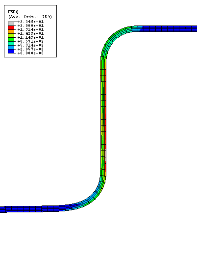
Figure 3. Equivalent plastic strain PEEQ for speedup of 5 (mass scaling of 25).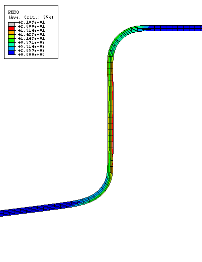
Figure 4. Kinetic and internal energy histories for mass scaling factors of 5, 10, and 25, corresponding to speedup factors of , , and 5, respectively.
- Discussion of speedup methods
-
As the mass scaling increases, the solution time decreases. The quality of the results also decreases because dynamic effects become more prominent, but there is usually some level of scaling that improves the solution time without sacrificing the quality of the results. Clearly, a speedup of 5 is too great to produce quasi-static results for this analysis.
A smaller speedup, such as , does not alter the results significantly. These results would be adequate for most applications, including springback analyses. With a scaling factor of 10 the quality of the results begins to diminish, while the general magnitudes and trends of the results remain intact. Correspondingly, the ratio of kinetic energy to internal energy increases noticeably. The results for this case would be adequate for many applications but not for accurate springback analysis.