How the mesh affects the stable time increment and CPU time | ||
| ||
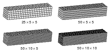
Table 1 shows how the CPU time (normalized with respect to the coarse mesh model result) changes with mesh refinement for this problem. The first half of the table provides the expected results, based on the simplified stability equations presented in this guide; the second half of the table provides the results obtained by running the analyses in Abaqus/Explicit on a desktop workstation.
| Mesh | Simplified Theory | Actual | ||||
|---|---|---|---|---|---|---|
| (s) | Number of Elements | CPU Time (s) | Max (s) | Number of Elements | Normalized CPU Time | |
| 25 × 5 × 5 | A | B | C | 5.754E-06 | 625 | 1 |
| 50 × 5 × 5 | A/2 | 2B | 4C | 2.954E-06 | 1250 | 4 |
| 50 × 10 × 5 | A/2 | 4B | 8C | 2.933E-06 | 2500 | 8.33 |
| 50 × 10 × 10 | A/2 | 8B | 16C | 2.907E-06 | 5000 | 16.67 |
For the theoretical results we choose the coarsest mesh, 25 × 5 × 5, as the base state, and we define the stable time increment, the number of elements, and the CPU time as variables A, B, and C, respectively. As the mesh is refined, two things happen: the smallest element dimension decreases, and the number of elements in the mesh increases. Each of these effects increases the CPU time. In the first level of refinement, the 50 × 5 × 5 mesh, the smallest element dimension is cut in half and the number of elements is doubled, increasing the CPU time by a factor of four over the previous mesh. However, further doubling the mesh to 50 × 10 × 5 does not change the smallest element dimension; it only doubles the number of elements. Therefore, the CPU time increases by only a factor of two over the 50 × 5 × 5 mesh. Further refining the mesh so that the elements are uniform and square in the 50 × 10 × 10 mesh again doubles the number of elements and the CPU time.
This simplified calculation predicts quite well the trends of how mesh refinement affects the stable time increment and CPU time. However, there are reasons why we did not compare the predicted and actual stable time increment values. First, recall that we made the approximation that the stable time increment is
We then assumed that the characteristic element length, , is the smallest element dimension, whereas Abaqus/Explicit actually determines the characteristic element length based on the overall size and shape of the element. Another complication is that Abaqus/Explicit employs a global stability estimator, which allows a larger stable time increment to be used. These factors make it difficult to predict the stable time increment accurately before running the analysis. However, since the trends follow nicely from the simplified theory, it is straightforward to predict how the stable time increment will change with mesh refinement.