Job diagnostics | ||
| ||
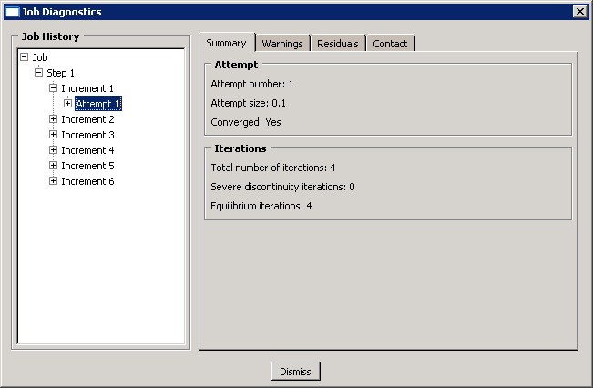
Enter the Visualization module, and open the output database file NlSkewPlate.odb to examine the convergence history. From the main menu bar, select to open the Job Diagnostics dialog box. Click the “” symbols in the Job History list to expand the list to include the steps, increments, attempts, and iterations in the analysis job. For example, under Increment 1, select Attempt 1, as shown in Figure 1.

The Attempt information on the right side of the dialog box contains basic information such as the increment size; the Iterations information contains the number of iterations attempted. Select Iteration 1 of this attempt to see detailed information regarding the first iteration. The information on the Summary tabbed page tells you that convergence was not achieved in this iteration, so click the Residuals tab to understand why.
As shown in Figure 2, the Residuals tabbed page displays the values of the average force, , and time average force, , in the model.

It also displays the values of the largest residual force, , the largest increment of displacement, , and the largest correction to displacement, , as well as the nodes and degrees of freedom (DOF) at which these occur. The location in the model where any of these occur can be highlighted in the viewport by toggling on Highlight selection in viewport at the bottom of the dialog box. The selection of the diagnostic criterion is persistent. Thus, you can click your way through the list of iterations on the left side of the dialog box to quickly see how the location associated with a given criterion changes throughout the iteration history. This may prove very useful if you are trying to debug a large, complex model. A similar display is available for rotational degrees of freedom (select Rotation under the list of Variables).
In this example the initial time increment is 0.1, as specified in the step definition. The average force for the increment is 12.2 N; and the time average force, , has the same value since this is the first increment. The largest residual force in the model, , is −749.6 N, which is clearly greater than 0.005 × . occurred at node 167 in degree of freedom 1 (your values and node numbers may vary). Abaqus/Standard must also check for equilibrium of the moments in the model since this model includes shell elements. The moment/rotation field also failed to satisfy the equilibrium check.
Although failure to satisfy the equilibrium check is enough to cause Abaqus/Standard to try another iteration, you should also examine the displacement correction. In the first iteration of the first increment of the first step the largest increment of displacement, , and the largest correction to displacement, , are both −5.578 × 10⁻³ m; and the largest increment of rotation and correction to rotation are both −1.598 × 10⁻² radians. Since the incremental values and the corrections are always equal in the first iteration of the first increment of the first step, the check that the largest corrections to nodal variables are less than 1% of the largest incremental values will always fail. However, if Abaqus/Standard judges the solution to be linear (a judgement based on the magnitude of the residuals, < 10−8), it will ignore this criterion.
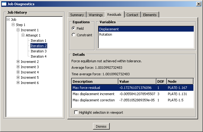
Since Abaqus/Standard did not find an equilibrium solution in the first iteration, it tries a second iteration. The residual information for the second iteration is shown in Figure 3.

In the second iteration has fallen to −0.173 N at node 167 in degree of freedom 1. However, equilibrium is not satisfied in this iteration because 0.005 × , where = 1.00 N, is still less than . The displacement correction criterion also failed again because = −7.055 × 10⁻⁵, which occurred at node 5 in degree of freedom 1, is more than 1% of = −5.584 × 10⁻³, the maximum displacement increment.
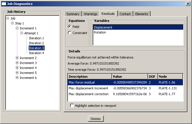
Both the moment residual check and the largest correction to rotation check were satisfied in this second iteration; however, Abaqus/Standard must perform two more iterations because the solutions did not pass the force residual check (or the largest correction to displacement criterion). The residual information for the additional iterations necessary to obtain a solution in the first increment are shown in Figure 4 and Figure 5.


After the fourth iteration = 0.997 N and = 1.794 × 10⁻⁷ N at node 76 in degree of freedom 1. These values satisfy < 0.005 × , so the force residual check is satisfied. Comparing to the largest increment of displacement shows that the displacement correction is below the required tolerance. The solution for the forces and displacements has, therefore, converged. The checks for both the moment residual and the rotation correction continue to be satisfied, as they have been since the second iteration. With a solution that satisfies equilibrium for all variables (displacement and rotation in this case), the first load increment is complete. The attempt summary (Figure 1) shows the number of iterations that were required for this increment and the size of the increment.
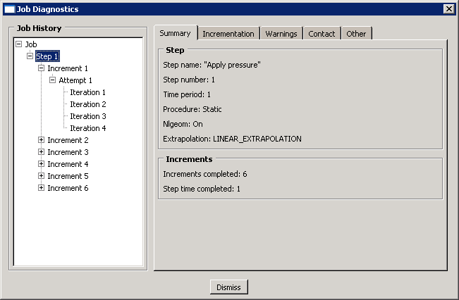
Abaqus/Standard continues this process of applying an increment of load then iterating to find a solution until it completes the whole analysis (or reaches the maximum increment that you specified). In this analysis it required five more increments. The step summary is shown in Figure 6.

In addition to the residual information discussed above, analysis warning messages related to numerical singularities, zero pivots, and negative eigenvalues, if they exist, are displayed in the Job Diagnostics dialog box (in the Warnings tabbed page). Always investigate the cause of these warnings.