Postprocessing the results

Create a plot of the model's deformed shape, and check that this shape is realistic.

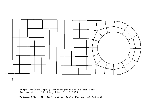
The default view is isometric. You can set the view shown in Figure 1 by using the options in the View menu or the tools in the View Manipulation toolbar; in this figure perspective is also turned off.

Figure 1. Deformed model shape using results for the simulation without hardening.

The displacements and, particularly, the rotations of the lug shown in the plot are large but do not seem large enough to have caused all of the numerical problems seen in the simulation. Look closely at the information in the plot's title for an explanation. The deformation scale factor used in this plot is 0.02; i.e., the displacements are scaled to 2% of their actual values. (Your deformation scale factor may be different.)

Abaqus/CAE always scales the displacements in a geometrically linear simulation such that the deformed shape of the model fits into the viewport. (This is in contrast to a geometrically nonlinear simulation, where Abaqus/CAE does not scale the displacements and, instead, adjusts the view by zooming in or out to fit the deformed shape in the plot.) To plot the actual displacements, set the deformation scale factor to 1.0. This will produce a plot of the model in which the lug has deformed until it is almost parallel to the vertical (global Y) axis.

The applied load of 60 kN exceeds the limit load of the lug, and the lug collapses when the material yields at all the integration points through its thickness. The lug then has no stiffness to resist further deformation because of the perfectly plastic post-yield behavior of the steel. This is consistent with the pattern observed earlier concerning the locations of the large strain increments and maximum displacement corrections.