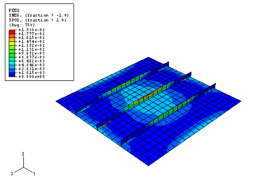
Postprocessing | ||
| ||
- Changing the view
The default view is isometric, which does not provide a particularly clear view of the plate. To improve the viewpoint, rotate the view using the options in the menu or the tools in the View Manipulation toolbar. Specify the view and select the viewpoint method for rotating the view. Enter the X-, Y-, and Z-coordinates of the viewpoint vector as 1,0.5,1 and the coordinates of the up vector as 0,1,0.
- Verifying shell section assignment
You can also visualize the section assignment and the shell thickness while postprocessing the results. For example, regions with common section assignments can be color coded to verify that the properties were assigned correctly (select Sections from the Color Code toolbar to color the mesh according to section assignment). To render the shell thickness, select from the main menu bar. In the ODB Display Options dialog box, toggle on Render shell thickness and click . If the model looks correct, as shown in Figure 1, toggle off this option and click before proceeding with the rest of the postprocessing instructions. Otherwise, correct the section assignment and rerun the job.
Figure 1. Plate with shell thickness displayed.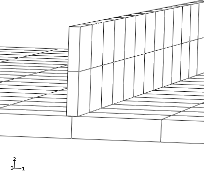
- Animation of results
As noted in earlier examples, animating your results will provide a general understanding of the dynamic response of the plate under the blast loading. First, plot the deformed model shape. Then, create a time-history animation of the deformed shape. Use the Animation Options dialog box to change the mode to Play once.
You will see from the animation that as the blast loading is applied, the plate begins to deflect. Over the duration of the load the plate begins to vibrate and continues to vibrate after the blast load has dropped to zero. The maximum displacement occurs at approximately 8 ms, and a displaced plot of that state is shown in Figure 2.
Figure 2. Displaced shape at 8 ms.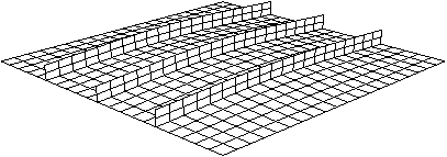
The animation images can be saved to a file for playback at a later time.
To save the animation:
From the main menu bar, select .
The Save Image Animation dialog box appears.
In the Settings field, enter the file name blast_base.
The format of the animation can be specified as AVI, QuickTime, VRML, or Compressed VRML.
Choose the QuickTime format, and click .
The animation is saved as blast_base.mov in your current directory. Once saved, your animation can be played external to Abaqus/CAE using industry-standard animation software.
- History output
Since it is not easy to see the deformation of the plate from the deformed plot, it is desirable to view the deflection response of the central node in the form of a graph. The displacement of the node in the center of the plate is of particular interest since the largest deflection occurs at this node.
Display the displacement history of the central node, as shown in Figure 3 (with displacements in millimeters).
Figure 3. Central node displacement as a function of time.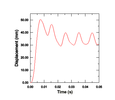
To generate a history plot of the central node displacement:
In the Results Tree, double-click the history output data named Spatial displacement: U2 at the node in the center of the plate (set Center).
Save the current X–Y data: in the Results Tree, click mouse button 3 on the data name and select Save As from the menu that appears. Name the data DISP.
The units of the displacements in this plot are meters. Modify the data to create a plot of displacement (in millimeters) versus time by creating a new data object.
In the Results Tree, expand the XYData container.
The DISP data are listed underneath.
In the Results Tree, double-click XYData; then select in the Create XY Data dialog box. Click .
In the Operate on XY Data dialog box, multiply DISP by 1000 to create the plot with the displacement values in millimeters instead of meters. The expression at the top of the dialog box should appear as:
"DISP" * 1000
Click to see the modified X–Y data. Save the data as U2_BASE.
Close the Operate on XY Data dialog box.
Click the Axis Options
 tool in the toolbox. In the Axis Options dialog box, change the X-axis title to Time (s) and the Y-axis title to Displacement (mm). Click to close the dialog box. The resulting plot is shown in Figure 3.
The plot shows that the displacement reaches a maximum of 50.2 mm at 7.7 ms and then oscillates after the blast load is removed.
The other quantities saved as history output in the output database are the total energies of the model. The energy histories can help identify possible shortcomings in the model as well as highlight significant physical effects. Display the histories of five different energy output variables—ALLAE, ALLIE, ALLKE, ALLPD, and ALLSE.
To generate history plots of the model energies:
Save the history results for the ALLAE, ALLIE, ALLKE, ALLPD, and ALLSE output variables as X–Y data. A default name is given to each curve; rename each according to its output variable name: ALLAE, ALLKE, etc.
In the Results Tree, expand the XYData container.
The ALLAE, ALLIE, ALLKE, ALLPD, and ALLSE X–Y data objects are listed underneath.
Select ALLAE, ALLIE, ALLKE, ALLPD, and ALLSE using Ctrl; click mouse button 3, and select from the menu that appears to plot the energy curves.
To more clearly distinguish between the different curves in the plot, open the Curve Options dialog box and change their line styles.
-
For the curve ALLSE, select a dashed line style.
-
For the curve ALLPD, select a dotted line style.
-
For the curve ALLAE, select a chain dashed line style.
-
For the curve ALLIE, select the second thinnest line type.
-
To change the position of the legend, open the Chart Legend Options dialog box and switch to the Area tabbed page.
In the Position region of this page, toggle on Inset and click Dismiss. Drag the legend in the viewport so that it fits within the grid, as shown in Figure 4.
Figure 4. Energy quantities as a function of time.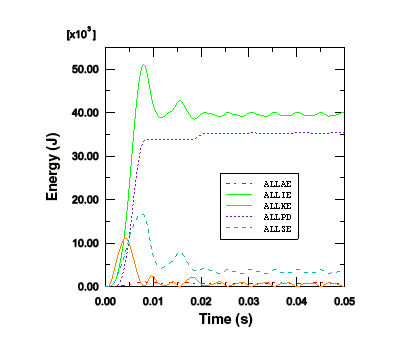
We can see that once the load has been removed and the plate vibrates freely, the kinetic energy increases as the strain energy decreases. When the plate is at its maximum deflection and, therefore, has its maximum strain energy, it is almost entirely at rest, causing the kinetic energy to be at a minimum.
The plastic strain energy rises to a plateau and then rises again. From the plot of kinetic energy we can see that the second rise in plastic strain energy occurs when the plate has rebounded from its maximum displacement and is moving back in the opposite direction. We are, therefore, seeing plastic deformation on the rebound after the blast pulse.
Even though there is no indication that hourglassing is a problem in this analysis, study the artificial strain energy to make sure. As discussed in Using Continuum Elements, artificial strain energy or “hourglass stiffness” is the energy used to control hourglass deformation, and the output variable ALLAE is the accumulated artificial strain energy. This discussion on hourglass control applies equally to shell elements. Since energy is dissipated as plastic deformation as the plate deforms, the total internal energy is much greater than the elastic strain energy alone. Therefore, it is most meaningful in this analysis to compare the artificial strain energy to an energy quantity that includes the dissipated energy as well as the elastic strain energy. Such a variable is the total internal energy, ALLIE, which is a summation of all internal energy quantities. The artificial strain energy is approximately 2% of the total internal energy, indicating that hourglassing is not a problem.
One thing we can notice from the deformed shape is that the central stiffener is subject to almost pure in-plane bending. Using only two first-order, reduced-integration elements through the depth of the stiffener is not sufficient to model in-plane bending behavior. While the solution from this coarse mesh appears to be adequate since there is little hourglassing, for completeness we will study how the solution changes when we refine the mesh of the stiffener. Use caution when you refine the mesh, since mesh refinement will increase the solution time by increasing the number of elements and decreasing the element size.
Edit the mesh, and respecify the mesh density. Using the previously saved edge set, specify four elements through the height of each stiffener, and remesh the part instance. Create a new job named BlastLoadRefined. Submit this job for analysis, and investigate the results when the job has completed running.
This increase in the number of elements increases the solution time by approximately 20%. In addition, the stable time increment decreases by approximately a factor of two as a result of the reduction of the smallest element dimension in the stiffeners. Since the total increase in solution time is a combination of the two effects, the solution time of the refined mesh increases by approximately a factor of 1.2 × 2, or 2.4, over that of the original mesh.
Figure 5 shows the histories of artificial energy for both the original mesh and the mesh with the refined stiffeners. The artificial energy is slightly lower in the refined mesh. As a result, we would not expect the results to change significantly from the original to the refined mesh.
Figure 5. Artificial energy in the original and refined meshes.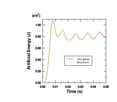
Figure 6 shows that the displacement of the plate's central node is almost identical in both cases, indicating that the original mesh is capturing the overall response adequately. One advantage of the refined mesh, however, is that it better captures the variation of stress and plastic strain through the stiffeners.
Figure 6. Central node displacement history for the original and refined meshes.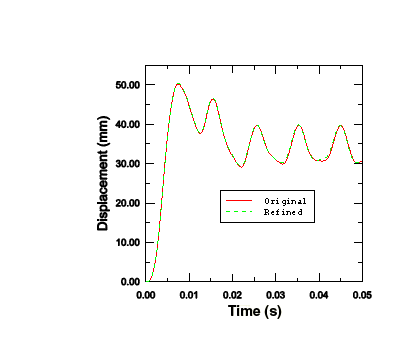
- Contour plots
In this section you will use the contour plotting capability of the Visualization module to display the von Mises stress and equivalent plastic strain distributions in the plate. Use the model with the refined stiffener mesh to create the plots; from the main menu bar, select and choose the file BlastLoadRefined.odb.
To generate contour plots of the von Mises stress and equivalent plastic strain:
From the list of variable types on the left side of the Field Output toolbar, select Primary.
From the list of output variables in the center of the toolbar, select S. The stress invariants and components are available in the next list to the right. Select the Mises stress invariant.
From the main menu bar, select .
In the Section Points dialog box that appears, select Top and bottom as the active locations and click .
Select , or use the
 tool from the toolbox.
Abaqus plots the contours of the von Mises stress on both the top and bottom faces of each shell element. To see this more clearly, rotate the model in the viewport.
The view that you set earlier for the animation exercise should be changed so that the stress distribution is clearer.
Change the view back to the default isometric view using the
 tool in the Views toolbar.
Tip: If the Views toolbar is not visible, select from the main menu bar. Figure 7 shows a contour plot of the von Mises stress at the end of the analysis.
Figure 7. Contour plot of von Mises stress at 50 ms.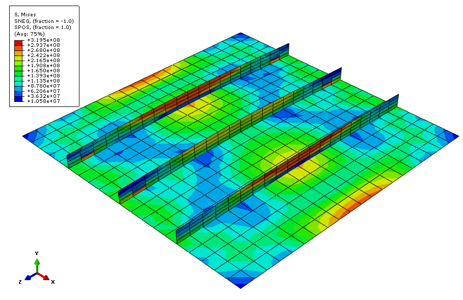
Similarly, contour the equivalent plastic strain. Select Primary from the list of variable types on the left side of the Field Output toolbar and select PEEQ from the list of output variables next to it.
Figure 8 shows a contour plot of the equivalent plastic strain at the end of the analysis.
Figure 8. Contour plot of equivalent plastic strain at 50 ms.