Postprocessing the dynamic analysis results

Open the output database (.odb) file created by this job.

Plotting the deformed shape

From the main menu bar, select PlotDeformed Shape; or use the tool in the toolbox. Figure 1 displays the deformed model shape at the end of the analysis.

Figure 1. Deformed model shape for the explicit analysis (shaded).

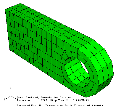
As discussed earlier, Abaqus/Explicit assumes large deformation theory by default; thus, the deformation scale factor is automatically set to 1. If the displacements are too small to be seen, scaling can be applied to aid the study of the response.

To see the vibrations in the lug more clearly, change the deformation scale factor to 50. In addition, animate the time history of the deformed shape of the lug and decrease the frame rate of the time history animation.

The time history animation of the deformed shape of the lug shows that the suddenly applied load induces vibrations in the lug. Additional insights about the behavior of the lug under this type of loading can be gained by plotting the kinetic energy, internal energy, displacement, and stress in the lug as a function of time. Some of the questions to consider are:

1. Is energy conserved?

2. Was large-displacement theory necessary for this analysis?

3. Are the peak stresses reasonable? Will the material yield?

X–Y plotting

X–Y plots can display the variation of a variable as a function of time. You can create X–Y plots from field and history output.

To create X–Y plots of the internal and kinetic energy as a function of time:

1. In the Results Tree, expand the History Output container underneath the output database named expLug.odb.

2. The list of all the variables in the history portion of the output database appears; these are the only history output variables you can plot.

   From the list of available output variables, double-click ALLIE to plot the internal energy for the whole model.

   Abaqus reads the data for the curve from the output database file and plots the graph shown in Figure 2.

   Figure 2. Internal energy for the whole model.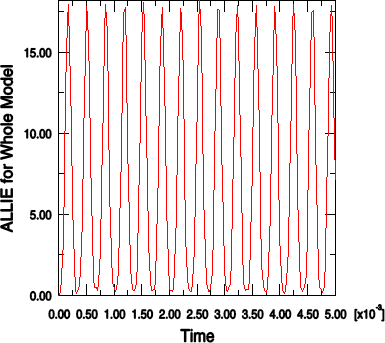
   
   

3. Repeat this procedure to plot ALLKE, the kinetic energy for the whole model (shown in Figure 3).

   Figure 3. Kinetic energy for the whole model.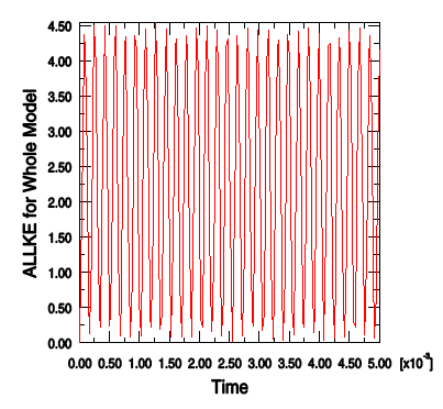
   
   

   Both the internal energy and the kinetic energy show oscillations that reflect the vibrations of the lug. Throughout the simulation, kinetic energy is transformed into internal (strain) energy and vice-versa. Since the material is linear elastic, total energy is conserved. This can be seen by plotting ETOTAL, the total energy of the system, together with ALLIE and ALLKE. The value of ETOTAL is approximately zero throughout the course of the analysis. Energy balances in dynamic analysis are discussed further in Nonlinear Explicit Dynamics.

We will examine the nodal displacements at the bottom of the lug hole to evaluate the significance of geometrically nonlinear effects in this simulation.

To generate a plot of displacement versus time:

1. Plot the deformed shape of the lug. In the Results Tree, double-click XY Data.

2. In the Create XY Data dialog box that appears, select ODB field output as the source and click Continue.

3. In the XY Data from ODB Field Output dialog box that appears, select Unique Nodal as the type of position from which the X–Y data should be read.

4. Click the arrow next to U: Spatial displacement and toggle on U2 as the displacement variable for the X–Y data.

5. Select the Elements/Nodes tab. Choose Pick from viewport as the selection method for identifying the node for which you want X–Y data.

6. Click Edit Selection. In the viewport, select one of the nodes on the bottom of the hole as shown in Figure 4 (if necessary, change the render style to facilitate your selection). Click Done in the prompt area.

   Figure 4. Selected node at the bottom of the hole.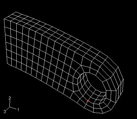
   
   

7. Click Plot in the XY Data from ODB Field Output dialog box to plot the nodal displacement as a function of time.

   The history of the oscillation, as shown in Figure 5, indicates that the displacements are small (relative to the structure's dimensions).

   Figure 5. Displacement of a node at the bottom of the hole.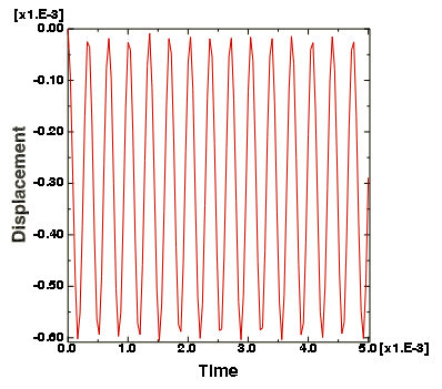
   
   

   Thus, this problem could have been solved adequately using small-deformation theory. This would have reduced the computational cost of the simulation without significantly affecting the results. Nonlinear geometric effects are discussed further in Nonlinearity.

We are also interested in the stress history of the connecting lug. The area of the lug near the built-in end is of particular interest because the peak stresses expected to occur there may cause yielding in the material.

To generate a plot of Mises stress versus time:

1. Plot the deformed shape of the lug again.

2. Select the Variables tab in the XY Data from ODB Field Output dialog box. Deselect U2 as the variable for the X–Y data plot.

3. Change the Position field to Integration Point.

4. Click the arrow next to S: Stress components and toggle on Mises as the stress variable for the X–Y data.

5. Select the Elements/Nodes tab. Choose Pick from viewport as the selection method for identifying the element for which you want X–Y data.

6. Click Edit Selection. In the viewport, select one of the elements near the built-in end of the lug as shown in Figure 6. Click Done in the prompt area.

   Figure 6. Selected element near the built-in end of the lug.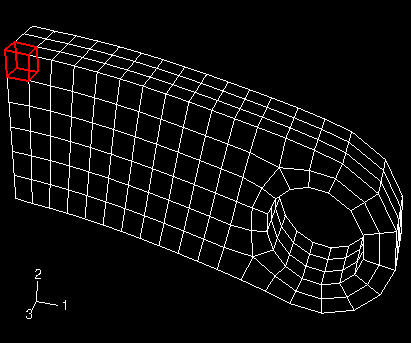
   
   

7. Click Plot in the XY Data from ODB Field Output dialog box to plot the Mises stress at the selected element as a function of time.

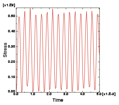
The peak Mises stress is on the order of 550 MPa, as shown in Figure 7. This value is larger than the typical yield strength of steel. Thus, the material would have yielded before experiencing such a large stress state. Material nonlinearity is discussed further in Materials.

Figure 7. Mises stress near the built-in end of the lug.