Mesh convergence | ||
| ||
As you gain experience, you will learn to judge what level of refinement produces a suitable mesh to give acceptable results for most simulations. However, it is always good practice to perform a mesh convergence study, where you simulate the same problem with a finer mesh and compare the results. You can have confidence that your model is producing a mathematically accurate solution if the two meshes give essentially the same result.
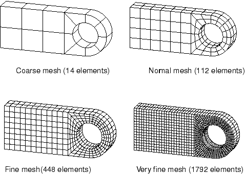
Mesh convergence is an important consideration in both Abaqus/Standard and Abaqus/Explicit. The connecting lug will be used as an example of a mesh refinement study by further analyzing the connecting lug in Abaqus/Standard using four different mesh densities (Figure 1). The number of elements used in each mesh is indicated in the figure.
Note:
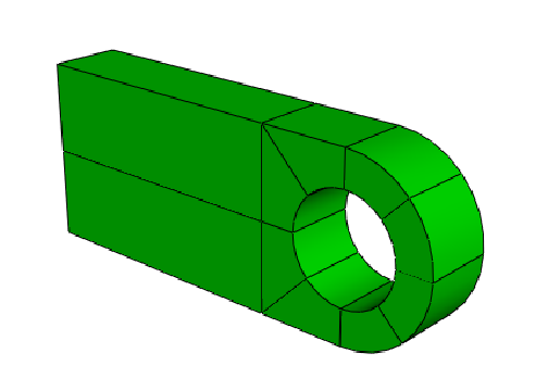
The meshes in Figure 1 can be obtained by further partitioning, as indicated in Figure 2, with appropriate mesh seeding.
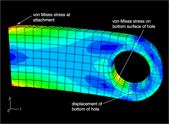
We consider the influence of the mesh density on three particular results from this model:
The displacement of the bottom of the hole.
The peak Mises stress at the stress concentration on the bottom surface of the hole.
The peak Mises stress where the lug is attached to the parent structure.
The locations where the results are compared are shown in Figure 3.
The results for each of the four mesh densities are compared in Table 1, along with the CPU time required to run each simulation.
| Mesh | Displacement of bottom of hole | Stress at bottom of hole | Stress at attachment | Relative CPU time |
|---|---|---|---|---|
| Coarse | 3.07E−4 | 256.E6 | 312.E6 | 0.83 |
| Normal | 3.13E−4 | 311.E6 | 365.E6 | 1.0 |
| Fine | 3.14E−4 | 332.E6 | 426.E6 | 3.2 |
| Very fine | 3.15E−4 | 345.E6 | 496.E6 | 13.3 |
The coarse mesh predicts less accurate displacements at the bottom of hole, but the normal, fine, and very fine meshes all predict similar results. The normal mesh is, therefore, converged as far as the displacements are concerned. The convergence of the results is plotted in Figure 4.
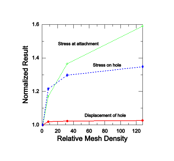
All the results are normalized with respect to the values predicted by the coarse mesh. The peak stress on the bottom of the hole converges much more slowly than the displacements because stress and strain are calculated from the displacement gradients; thus, a much finer mesh is required to predict accurate displacement gradients than is needed to calculate accurate displacements.
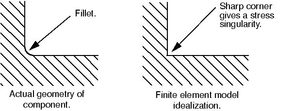
Mesh refinement significantly changes the stress calculated at the attachment of the connecting lug; it continues to increase with continued mesh refinement. A stress singularity exists at the corner of the lug where it attaches to the parent structure. Theoretically the stress is infinite at this location; therefore, increasing the mesh density will not produce a converged stress value at this location. This singularity occurs because of the idealizations used in the finite element model. The connection between the lug and the parent structure has been modeled as a sharp corner, and the parent structure has been modeled as rigid. These idealizations lead to the stress singularity. In reality there probably will be a small fillet between the lug and the parent structure, and the parent structure will be deformable, not rigid. If the exact stress in this location is required, the fillet between the components must be modeled accurately (see Figure 5) and the stiffness of the parent structure must also be considered.
It is common to omit small details like fillet radii from a finite element model to simplify the analysis and to keep the model size reasonable. However, the introduction of any sharp corner into a model will lead to a stress singularity at that location. This normally has a negligible effect on the overall response of the model, but the predicted stresses close to the singularity will be inaccurate.
For complex, three-dimensional simulations the available computer resources often dictate a practical limit on the mesh density that you can use. In this case you must use the results from the analysis carefully. Coarse meshes are often adequate to predict trends and to compare how different concepts behave relative to each other. However, you should use the actual magnitudes of displacement and stress calculated with a coarse mesh with caution.
It is rarely necessary to use a uniformly fine mesh throughout the structure being analyzed. You should use a fine mesh mainly in the areas of high stress gradients and use a coarser mesh in areas of low stress gradients or where the magnitude of the stresses is not of interest. For example, Figure 6 shows a mesh that is designed to give an accurate prediction of the stress concentration at the bottom of the hole.
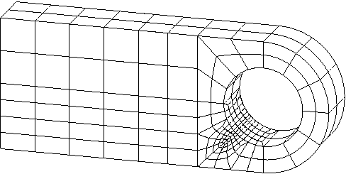
A fine mesh is used only in the region of high stress gradients, and a coarse mesh is used elsewhere. The results from an Abaqus/Standard simulation with this locally refined mesh are shown in Table 2. This table shows that the results are comparable to those from the very fine mesh, but the simulation with the locally refined mesh required considerably less CPU time than the analysis with the very fine mesh.
| Mesh | Displacement of bottom of hole | Stress at bottom of hole | Relative CPU time |
|---|---|---|---|
| Very fine | 3.15E−4 | 345.E6 | 22.5 |
| Locally refined | 3.14E−4 | 346.E6 | 3.44 |
You can often predict the locations of the highly stressed regions of a model—and, hence, the regions where a fine mesh is required—using your knowledge of similar components or with hand calculations. This information can also be gained by using a coarse mesh initially to identify the regions of high stress and then refining the mesh in these regions. The latter procedure is carried out easily using preprocessors like Abaqus/CAE where the complete numerical model (i.e., material properties, boundary conditions, loads, etc.) can be defined based on the geometry of the structure. It is simple to mesh the geometry coarsely for the initial simulation and then to refine the mesh in the appropriate regions, as indicated by the results from the coarse simulation.
Abaqus provides an advanced feature, called submodeling, that allows you to obtain more detailed (and accurate) results in a region of interest in the structure. The solution from a coarse mesh of the entire structure is used to “drive” a detailed local analysis that uses a fine mesh in this region of interest. (This topic is beyond the scope of this guide. See About submodeling, for further details.)