Riser dynamics

This example verifies the response of a riser under different types of load conditions.

Pipelines extending from the sea floor to the ocean surface (risers) are subject to many types of load: self-weight, buoyancy, internal and external pressure, tensile forces arising from surface moorings, current drag, and oscillatory loads resulting from wave motion. The response of a riser to these loads is complex, and the difficulty of such analysis is heightened by the relative length of such pipelines (deep water risers). In this example a riser is analyzed under conditions specified by the American Petroleum Institute for comparison of drilling riser analyses (API BULLETIN2J, 1977), and the results are compared with the results shown in that publication.

The following topics are discussed:

Geometry and model
Loading
Boundary conditions
Analysis
Results and discussion
Input files
References
Figures

ProductsAbaqus/StandardAbaqus/Aqua

Geometry and model

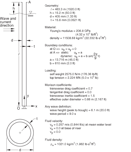
The riser is shown in Figure 1. Its length is 463.3 m (1520 ft), and it stands in 448.1 m (1470 ft) of water. The outer diameter of the riser is 405 mm (1.33 ft), and it has a wall thickness of 15.88 mm (0.0521 ft). The pipeline is made of steel, with a Young's modulus of 206.8 GPa (4.32 × 10⁹ lb/ft²) and a density of 11508.685 kg/m³ (22.332 lb-s²/ft⁴). The riser is modeled with 10 beam elements of type B21. No mesh convergence studies have been performed; hence, more elements may be required for accurate prediction of the stress in the riser.

Loading

The riser has a weight of 2575 N/m (176.36 lb/ft) and is loaded by a top tension of 2.224 MN (5 × 10⁵ lb). Drag loading is applied by a steady current flowing by the riser with a velocity distribution varying linearly from 0.257 m/s (0.844 ft/s) at the mean water level to zero at the base of the riser. The coefficients in Morison's equation are transverse drag coefficient ( $C_{D}$ ) 0.7, tangential drag coefficient ( $C_{T}$ ) 0.0, and transverse inertia coefficient ( $C_{M}$ ) 1.5.

The effective outer diameter for the drag calculations is 0.66 m (2.167 ft). Waves of peak to trough height 6.1 m (20 ft) travel across the water surface with a period of 9 seconds; these are modeled with the Airy wave theory provided in Abaqus/Aqua (Abaqus/Aqua analysis). The density of the fluid is taken to be 1021 kg/m³ (1.982 lb–s²/ft⁴). In Abaqus/Aqua, user subroutine UWAVE can be used to specify user-defined wave kinematics. We illustrate this capability by repeating this analysis with a user-specified Airy wave theory that is identical to the built-in Airy wave option in Abaqus/Aqua.

Boundary conditions

The base of the riser is “gimballed,” supporting no moments. The top of the riser has two motions prescribed: an initial offset of 13.716 m (45 ft) from the vertical position of the riser and a sinusoidal motion about this static configuration, representing the surge of a vessel attached to the riser, with peak-to-peak amplitude of 1.22 m (4 ft) and a period of 9 seconds. The vessel surge angle is 15° out of phase with the surface waves. The phase angle, $ϕ_{N}$ , for the Airy wave definition provides an arbitrary choice of origin in time for the vertical displacement of a fluid particle. Based on the initial offset and vessel surge angle, this angle is set to −54.026°, where the negative sign indicates that the wave lags behind the vessel surge.

Analysis

The analysis is done in two steps. The first is the static step, in which the top tension is applied and the riser is moved from the vertical to its offset position by specifying the necessary horizontal displacement at the top of the pipeline. The top tension is 2.224 MN (5 × 10⁵ lb).

In the second step, which is a dynamic step, the time increment is chosen as a fixed value of 0.125 second. The prescribed displacement at the top of the riser has a 9-second period, so this time step should provide reasonably accurate time integration once the higher modes are damped out by the fluid drag. The “half-increment residual” values calculated by Abaqus provide a measure of accuracy of the solution, and these values are typically of order 4.4 kN (1000 lb). Since these values are smaller than typical actual forces, they suggest that the time integration is reasonably accurate.

Results and discussion

The initial static step, which moves the riser to its offset position and applies the static loads, is completed in four increments. The first increment requires more iterations than subsequent increments, which is typical of this class of problem: the riser is initially unstressed and, therefore, is highly flexible. After some loading is applied, the axial tension stabilizes the system, and convergence is more rapid.

At the end of the static step the top of the riser makes an angle of 1.17° with the vertical. This value agrees well with the value of 1.20° presented in API BULLETIN2J (1977). The angle predicted at the base of the riser is 2.48°, which compares to 2.55° reported in the API bulletin. The slight discrepancies are attributed to the relative coarseness of the model.

The dynamic solution is carried out for 18 seconds of response. Typically one equilibrium iteration is required in each of the time increments. Half-increment residual values for the first few increments are of order 178 MN (4.0 × 10⁷ lb), and at the end of the run they are of order 4.4 kN (1000 lb). This result is typical: initially there is much high frequency content in the solution, which is reflected in the larger half-increment residual values. As the analysis proceeds, the fluid drag dissipates this “noise,” the solution becomes smoother, and the half-increment residual values drop accordingly.

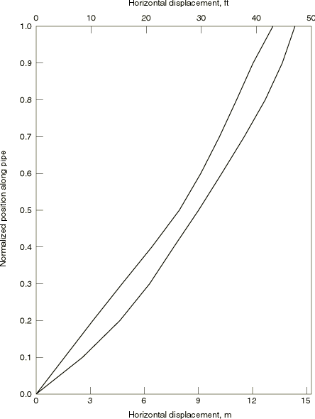
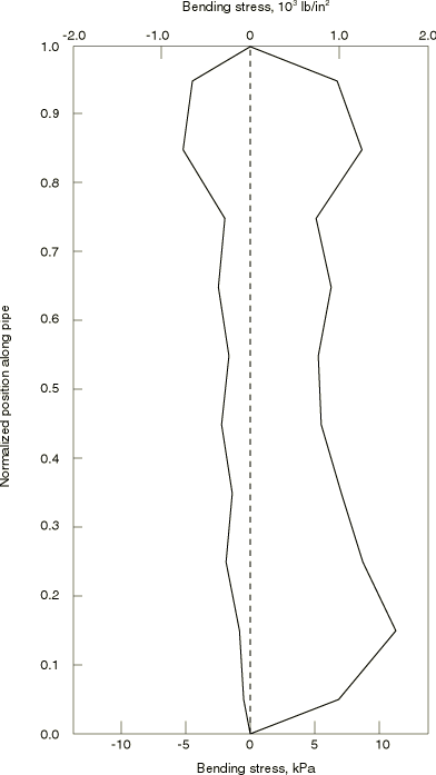
The envelope of pipeline excursions during the second cycle of the dynamic excitation is plotted in Figure 2, and the envelope of bending stress is shown in Figure 3. These results are in basic agreement with those given in the API bulletin.

As expected, the results obtained by the model with the Airy wave theory implemented in user subroutine UWAVE are identical to those due to the built-in Airy wave option.

Input files

riserdynamics_airy_disp.inp: Analysis with the Airy wave theory. User subroutine DISP is used to prescribe the sinusoidal surge motion. This motion could be prescribed instead through the use of the AMPLITUDE option. User subroutine DISP is used to illustrate the use of this routine to prescribe a nonzero boundary condition value.
riserdynamics_airy_disp.f: User subroutine DISP used in riserdynamics_airy_disp.inp.
riserdynamics_wavedata.inp: Wave data for use in riserdynamics_airy_disp.inp.
riserdynamics_stokes_disp.inp: Analysis with the Stokes wave theory.
riserdynamics_stokes_disp.f: User subroutine DISP used in riserdynamics_stokes_disp.inp.
riserdynamics_airy_disp_uwave.inp: Analysis with the Airy wave theory implemented in user subroutine UWAVE.
riserdynamics_airy_disp_uwave.f: User subroutines UWAVE and DISP used in riserdynamics_airy_disp_uwave.inp.
exa_riserdynamics_stokes_disp_uwave.inp: Analysis with the Stokes wave theory implemented in user subroutine UWAVE.
exa_riserdynamics_stokes_disp_uwave.f: User subroutines UWAVE and DISP used in exa_riserdynamics_stokes_disp_uwave.inp.

References

American Petroleum Institute, “Comparison of Marine Drilling Riser Analyses,” API Bulletin 2J, Washington, DC, January 1977.

Figures

Figure 1. Riser problem definition.

Figure 2. Horizontal displacement envelope during the second cycle of the dynamic excitation.

Figure 3. Bending stress envelope during the second cycle of the dynamic excitation.