Laminated composite shells: buckling of a cylindrical panel with a circular hole

This example illustrates modeling a thin, laminated composite shell in the presence of buckling.

The following topics are discussed:

Geometry and model
Relation between stress resultants and generalized strains
Results and discussion
Input files
References
Tables
Figures

ProductsAbaqus/Standard

The objective is to determine the strength of a thin, laminated composite shell, typical of shells used to form the outer surfaces of aircraft fuselages and rocket motors. Such analyses are complicated by the fact that these shells typically include local discontinuities—stiffeners and cutouts—which can induce substantial stress concentrations that can delaminate the composite material. In the presence of buckling this delamination can propagate through the structure to cause failure. In this example we study only the geometrically nonlinear behavior of the shell: delamination or other section failures are not considered. Some estimate of the possibility of material failure could presumably be made from the stresses predicted in the analyses reported here, but no such assessment is included in this example.

The example makes extensive use of material orientation in a general shell section to define the multilayered, anisotropic, laminated section. The various orientation options for shells are discussed in Analysis of an anisotropic layered plate.

General shell sections offer two methods of defining laminated sections: defining the thickness, material, and orientation of each layer or defining the equivalent section properties directly. The last method is particularly useful if the laminate properties are obtained directly from experiments or a separate preprocessor. This example uses both methods with a general shell section definition. Alternatively, you could use a shell section to analyze the model; however, because the material behavior is linear, no difference in solution would be obtained and the computational costs would be greater.

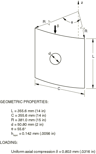
Geometry and model

The structure analyzed is shown in Figure 1 and was originally studied experimentally by Knight and Starnes (1984). The test specimen is a cylindrical panel with a 355.6 mm (14 in) square platform and a 381 mm (15 in) radius of curvature, so that the panel covers a 55.6° arc of the cylinder. The panel contains a centrally located hole of 50.8 mm (2 in) diameter. The shell consists of 16 layers of unidirectional graphite fibers in an epoxy resin. Each layer is 0.142 mm (.0056 in) thick. The layers are arranged in the symmetric stacking sequence { $\pm$ 45/90/0/0/90/ $\mp$ 45} degrees repeated twice. The nominal orthotropic elastic material properties as defined by Stanley (1985) are

$E_{11}$ = 135 kN/mm²		(19.6 × 10⁶ lb/in²),
$E_{22}$ = 13 kN/mm²		(1.89 × 10⁶ lb/in²),
$G_{12} = G_{13}$ = 6.4 kN/mm²		(.93 × 10⁶ lb/in²),
$G_{23}$ = 4.3 kN/mm²		(0.63 × 10⁶ lb/in²),
$ν_{12}$ = 0.38,

where the 1-direction is along the fibers, the 2-direction is transverse to the fibers in the surface of the lamina, and the 3-direction is normal to the lamina.

The panel is fully clamped on the bottom edge, clamped except for axial motion on the top edge and simply supported along its vertical edges. Three analyses are considered. The first is a linear (prebuckling) analysis in which the panel is subjected to a uniform end shortening of 0.8 mm (.0316 in). The total axial force and the distribution of axial force along the midsection are used to compare the results with those obtained by Stanley (1985). The second analysis consists of an eigenvalue extraction of the first five buckling modes. The buckling loads and mode shapes are also compared with those presented by Stanley (1985). Finally, a nonlinear load-deflection analysis is done to predict the postbuckling behavior, using the modified Riks algorithm. For this analysis an initial imperfection is introduced. The imperfection is based on the fourth buckling mode extracted during the second analysis. These results are compared with those of Stanley (1985) and with the experimental measurements of Knight and Starnes (1984).

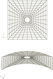
The mesh used in Abaqus is shown in Figure 2. The anisotropic material behavior precludes any symmetry assumptions, hence the entire panel is modeled. The same mesh is used with the 4-node shell element (type S4R5) and also with the 9-node shell element (type S9R5); the 9-node element mesh, thus, has about four times the number of degrees of freedom as the 4-node element mesh. The 6-node triangular shell element STRI65 is also used; it employs two triangles for each quadrilateral element of the second-order mesh. Mesh generation is facilitated by specifying node fill and node mapping, as shown in the input data. In this model specification of the relative angle of orientation to define the material orientation within each layer, along with orthotropic elasticity in plane stress, makes the definition of the laminae properties straightforward.

The shell elements used in this example use an approximation to thin shell theory, based on a numerical penalty applied to the transverse shear strain along the element edges. These elements are not universally applicable to the analysis of composites since transverse shear effects can be significant in such cases and these elements are not designed to model them accurately. Here, however, the geometry of the panel is that of a thin shell; and the symmetrical lay-up, along with the relatively large number of laminae, tends to diminish the importance of transverse shear deformation on the response.

Relation between stress resultants and generalized strains

The shell section is most easily defined by giving the layer thickness, material, and orientation, in which case Abaqus preintegrates to obtain the section stiffness properties. However, the user can choose to input the section stiffness properties directly instead, as follows.

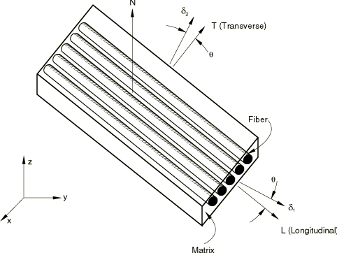
In Abaqus a lamina is considered as an orthotropic sheet in plane stress. The principal material axes of the lamina (see Figure 3) are longitudinal, denoted by L; transverse to the fiber direction in the surface of the lamina, denoted by T; and normal to the lamina surface, denoted by $N .$ The constitutive relations for a general orthotropic material in the principal directions ( $L, T, N$ ) are

{\begin{matrix} σ_{L} \\ σ_{T} \\ τ_{L T} \\ σ_{N} \\ τ_{L N} \\ τ_{T N} \end{matrix}} = [\begin{matrix} C_{11} & C_{12} & 0 & C_{14} & 0 & 0 \\ C_{12} & C_{22} & 0 & C_{24} & 0 & 0 \\ 0 & 0 & C_{33} & 0 & 0 & 0 \\ C_{14} & C_{24} & 0 & C_{44} & 0 & 0 \\ 0 & 0 & 0 & 0 & C_{55} & 0 \\ 0 & 0 & 0 & 0 & 0 & C_{66} \end{matrix}] {\begin{matrix} ϵ_{L} \\ ϵ_{T} \\ γ_{L T} \\ ϵ_{N} \\ γ_{L N} \\ γ_{T N} \end{matrix}} .

In terms of the data required to define orthotropic elasticity by specifying terms in the elastic stiffness matrix in Abaqus these are

\begin{matrix} C_{11} & = D_{1111}, C_{12} = D_{1122}, C_{14} = D_{1133}, C_{22} = D_{2222} \\ C_{24} & = D_{2233}, C_{33} = D_{1212}, C_{44} = D_{3333}, C_{55} = D_{1313} \\ C_{66} & = D_{2323} \end{matrix}

This matrix is symmetric and has nine independent constants. If we assume a state of plane stress, then $σ_{N}$ is taken to be zero. This yields

{\begin{matrix} σ_{L} \\ σ_{T} \\ τ_{L T} \\ τ_{L N} \\ τ_{T N} \end{matrix}} = [\begin{matrix} Q_{11} & Q_{12} & 0 & 0 & 0 \\ Q_{12} & Q_{22} & 0 & 0 & 0 \\ 0 & 0 & Q_{33} & 0 & 0 \\ 0 & 0 & 0 & Q_{55} & 0 \\ 0 & 0 & 0 & 0 & Q_{66} \end{matrix}] {\begin{matrix} ϵ_{L} \\ ϵ_{T} \\ γ_{L T} \\ γ_{L N} \\ γ_{T N} \end{matrix}},

where

\begin{matrix} Q_{11} & = C_{11} - \frac{C_{14} C_{14}}{C_{44}}, \\ Q_{12} & = C_{12} - \frac{C_{24} C_{14}}{C_{44}}, \\ Q_{22} & = C_{22} - \frac{C_{24} C_{24}}{C_{44}}, \\ Q_{33} & = C_{33}, \\ Q_{55} & = C_{55}, \\ Q_{66} & = C_{66} . \end{matrix}

The correspondence between these terms and the usual engineering constants that might be given for a simple orthotropic layer in a laminate is

\begin{matrix} Q_{11} & = \frac{E_{1}}{1 - ν_{12} ν_{21}}, \\ Q_{12} & = \frac{ν_{12} E_{2}}{1 - ν_{12} ν_{21}} = \frac{ν_{21} E_{1}}{1 - ν_{12} ν_{21}}, \\ Q_{22} & = \frac{E_{2}}{1 - ν_{12} ν_{21}}, \\ Q_{33} & = G_{12}, \\ Q_{55} & = G_{13}, \\ Q_{66} & = G_{23} . \end{matrix}

The parameters used on the right-hand side of the above equation are those that must be provided as part of the definition of orthotropic elasticity in plane stress.

If the ( $1, 2, N$ ) system denotes the standard shell basis directions that Abaqus chooses by default, the local stiffness components must be rotated to this system to construct the lamina's contribution to the general shell section stiffness. Since $Q_{i j}$ represent fourth-order tensors, in the case of a lamina they are oriented at an angle $θ$ to the standard shell basis directions used in Abaqus. Hence, the transformation is

\begin{matrix} {\bar{Q}}_{11} & = Q_{11} \cos^{4} θ + 2 (Q_{12} + 2 Q_{33}) \sin^{2} θ \cos^{2} θ + Q_{22} \sin^{4} θ, \\ {\bar{Q}}_{12} & = (Q_{11} + Q_{22} - 4 Q_{33}) \sin^{2} θ \cos^{2} θ + Q_{12} (\sin^{4} θ + \cos^{4} θ), \\ {\bar{Q}}_{22} & = Q_{11} \sin^{4} θ + 2 (Q_{12} + 2 Q_{33}) \sin^{2} θ \cos^{2} θ + Q_{22} \cos^{4} θ, \\ {\bar{Q}}_{13} & = (Q_{11} - Q_{12} - 2 Q_{33}) \sin θ \cos^{3} θ + (Q_{12} - Q_{22} + 2 Q_{33}) \sin^{3} θ \cos θ, \\ {\bar{Q}}_{23} & = (Q_{11} - Q_{12} - 2 Q_{33}) \sin^{3} θ \cos θ + (Q_{12} - Q_{22} + 2 Q_{33}) \sin θ \cos^{3} θ, \\ {\bar{Q}}_{33} & = (Q_{11} + Q_{22} - 2 Q_{12} - 2 Q_{33}) \sin^{2} θ \cos^{2} θ + Q_{33} (\sin^{4} θ + \cos^{4} θ), \\ {\bar{Q}}_{55} & = Q_{55} \cos^{2} θ - Q_{66} \sin^{2} θ, \\ {\bar{Q}}_{56} & = Q_{55} \sin θ \cos θ - Q_{66} \sin θ \cos θ, \\ {\bar{Q}}_{66} & = Q_{55} \sin^{2} θ - Q_{66} \cos^{2} θ, \end{matrix}

where ${\bar{Q}}_{i j}$ are the stiffness coefficients in the standard shell basis directions used by Abaqus.

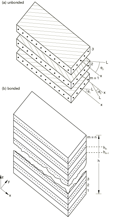
Abaqus assumes that a laminate is a stack of laminae arranged with the principal directions of each layer in different orientations. The various layers are assumed to be rigidly bonded together. The section force and moment resultants per unit length in the normal basis directions in a given layer can be defined on this basis as

\begin{matrix} (N_{1}, N_{2}, N_{12}) & = \int_{- h / 2}^{h / 2} (σ_{1}, σ_{2}, τ_{12}) d z, \end{matrix}

\begin{matrix} (M_{1}, M_{2}, M_{12}) & = \int_{- h / 2}^{h / 2} (σ_{1}, σ_{2}, τ_{12}) z d z, \\ (V_{1}, V_{2}) & = \int_{- h / 2}^{h / 2} (τ_{13}, τ_{23}) d z, \end{matrix}

where h is the thickness of the layer.

This leads to the relations

{\begin{matrix} N_{1} \\ N_{2} \\ N_{12} \\ M_{1} \\ M_{2} \\ M_{12} \\ V_{1} \\ V_{2} \end{matrix}} = [\begin{matrix} A_{11} & A_{12} & A_{13} & B_{11} & B_{12} & B_{13} & 0 & 0 \\ A_{12} & A_{22} & A_{23} & B_{12} & B_{22} & B_{23} & 0 & 0 \\ A_{13} & A_{23} & A_{33} & B_{13} & B_{23} & B_{33} & 0 & 0 \\ B_{11} & B_{12} & B_{13} & D_{11} & D_{12} & D_{13} & 0 & 0 \\ B_{12} & B_{22} & B_{23} & D_{12} & D_{22} & D_{23} & 0 & 0 \\ B_{13} & B_{23} & B_{33} & D_{13} & D_{23} & D_{33} & 0 & 0 \\ 0 & 0 & 0 & 0 & 0 & 0 & E_{11} & E_{12} \\ 0 & 0 & 0 & 0 & 0 & 0 & E_{12} & E_{22} \end{matrix}] {\begin{matrix} ϵ_{1} \\ ϵ_{2} \\ γ_{12} \\ κ_{1} \\ κ_{2} \\ κ_{12} \\ γ_{13} \\ γ_{23} \end{matrix}},

where the components of this section stiffness matrix are given by

\begin{matrix} (A_{i j}, B_{i j}, D_{i j}) & = \int_{- h / 2}^{h / 2} {\bar{Q}}_{i j}^{m} (1, z, z^{2}) d z, (i, j = 1, 2, 3) \\ E_{i j} & = \int_{- h / 2}^{h / 2} {\bar{Q}}_{α β}^{m} k_{i} k_{j} d z, (i, j = 1, 2, and α, β = i + 4, j + 4) . \end{matrix}

Here m indicates a particular layer. Thus, the ${\bar{Q}}_{i j}^{m}$ depend on the material properties and fiber orientation of the mth layer. The $k_{i}, i =$ 1,2 parameters are the shear correction coefficients as defined by Whitney (1973). If there are n layers in the lay-up, we can rewrite the above equations as a summation of integrals over the n laminae. The material coefficients will then take the form

\begin{matrix} A_{i j} & = \overset{n}{\sum_{m = 1}} {\bar{Q}}_{i j}^{m} (h_{m} - h_{m - 1}), \\ B_{i j} & = \frac{1}{2} \overset{n}{\sum_{m = 1}} {\bar{Q}}_{i j}^{m} (h_{m}^{2} - h_{m - 1}^{2}), \\ D_{i j} & = \frac{1}{3} \overset{n}{\sum_{m = 1}} {\bar{Q}}_{i j}^{m} (h_{m}^{3} - h_{m - 1}^{3}), \\ E_{i j} & = \overset{n}{\sum_{m = 1}} {\bar{Q}}_{α β}^{m} (h_{m} - h_{m - 1}) k_{i} k_{j}, \end{matrix}

where the $h_{m}$ and $h_{m - 1}$ in these equations indicate that the mth lamina is bounded by surfaces $z = h_{m}$ and $z = h_{m - 1} .$ See Figure 4 for the nomenclature.

These equations define the coefficients required for the direct input of the section stiffness matrix method in the general shell section. Only the $[A]$ , $[B]$ , and $[D]$ submatrices are needed for that option. The three terms in $[E]$ , if required, are defined as part of the transverse shear stiffness. The section forces as defined above are in the normal shell basis directions.

Applying these equations to the laminate defined for this example leads to the following overall section stiffness:

[A] = [\begin{matrix} 138.385 & 44.0189 & 0 \\ 44.0189 & 138.385 & 0 \\ 0 & 0 & 47.1831 \end{matrix}] kN/mm; [B] = [\begin{matrix} 0 & 0 & 0 \\ 0 & 0 & 0 \\ 0 & 0 & 0 \end{matrix}];

[D] = [\begin{matrix} 55.670 & 21.638 & 2.138 \\ 21.638 & 58.521 & 2.138 \\ 2.138 & 2.138 & 23.004 \end{matrix}] kN-mm; [E] = [\begin{matrix} 12.2387 & 0 \\ 0 & 12.2387 \end{matrix}] kN/mm,

[A] = [\begin{matrix} 790.239 & 251.367 & 0 \\ 251.367 & 790.239 & 0 \\ 0 & 0 & 269.436 \end{matrix}] \times 10^{3} lb/in; [B] = [\begin{matrix} 0 & 0 & 0 \\ 0 & 0 & 0 \\ 0 & 0 & 0 \end{matrix}];

[D] = [\begin{matrix} 492.719 & 191.513 & 18.9245 \\ 191.513 & 517.951 & 18.9245 \\ 18.9245 & 18.9245 & 203.602 \end{matrix}] lb-in; [E] = [\begin{matrix} 49.573 & 0.002 \\ 0.002 & 52.967 \end{matrix}] \times 10^{3} lb/in .

Results and discussion

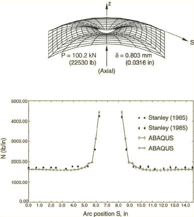
The total axial force necessary to compress the panel 0.803 mm (0.0316 in) is 100.2 kN (22529 lb) for the mesh of S9R5 elements, 99.5 kN (22359 lb) for the mesh of S4R5 elements, and 100.3 kN (22547 lb) for the mesh of STRI65 elements. These values match closely with the result of 100 kN (22480 lb) reported by Stanley (1985). Figure 5 shows the displaced configuration and a profile of axial force along the midsection of the panel (at $z = L / 2$ ). It is interesting to note that the axial load is distributed almost evenly across the entire panel, with only a very localized area near the hole subjected to an amplified stress level. This suggests that adequate results for this linear analysis could also be obtained with a coarser mesh that has a bias toward the hole.

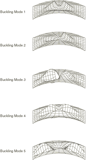
The second stage of the analysis is the eigenvalue buckling prediction. To obtain the buckling predictions with Abaqus, an eigenvalue buckling prediction step is run. In this step nominal values of load are applied. The magnitude that is used is not of any significance, since eigenvalue buckling is a linear perturbation procedure: the stiffness matrix and the stress stiffening matrix are evaluated at the beginning of the step without any of this load applied. The eigenvalue buckling prediction step calculates the eigenvalues that, multiplied with the applied load and added to any “base state” loading, are the predicted buckling loads. The eigenvectors associated with the eigenvalues are also obtained. This procedure is described in more detail in Eigenvalue buckling prediction.

The buckling predictions are summarized in Table 1 and Figure 6. The buckling load predictions from Abaqus are higher than those reported by Stanley. The eigenmode predictions given by the mesh using element types S4R5, S9R5, and STRI65 are all the same and agree well with those reported by Stanley. Stanley makes several important observations that remain valid for the Abaqus results: (1) the eigenvalues are closely spaced; (2) nevertheless, the mode shapes vary significantly in character; (3) the first buckling mode bears the most similarity to the linear prebuckling solution; (4) there is no symmetry available that can be utilized for computational efficiency.

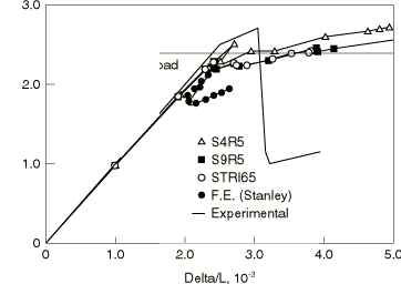
Following the eigenvalue buckling analyses, nonlinear postbuckling analysis is carried out by imposing an imperfection based on the fourth buckling mode. The maximum initial perturbation is 10% of the thickness of the shell. The load versus normalized displacement plots for the S9R5 mesh, the S4R5 mesh, and the STRI65 mesh are compared with the experimental results and those given by Stanley in Figure 7. The overall response prediction is quite similar for the Abaqus elements, although the general behavior predicted by Stanley is somewhat different. The Abaqus results show a peak load slightly above the buckling load predicted by the eigenvalue extraction, while Stanley's results show a significantly lower peak load. In addition, the Abaqus results show rather less loss of strength after the initial peak, followed quite soon by positive stiffness again. Neither the Abaqus results nor Stanley's results agree closely with the experimentally observed dramatic loss of strength after peak load. Stanley ascribes this to material failure (presumably delamination), which is not modeled in his analyses or in these.

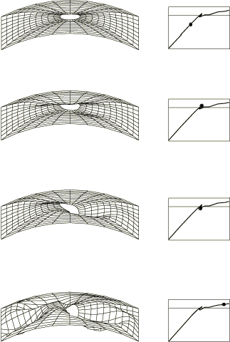
Figure 8 shows the deformed configurations for the panel during its postbuckling response. The plots show the results for S4R5, but the pattern is similar for S9R5 and STRI65. The response is quite symmetric initially; but, as the critical load is approached, a nonsymmetric dimple develops and grows, presumably accounting for the panel's loss of strength. Later in the postbuckling response another wrinkle can be seen to be developing.

Input files

laminpanel_s9r5_prebuckle.inp: Prebuckling analysis for the 9-node (element type S9R5) mesh.
laminpanel_s9r5_buckle.inp: Eigenvalue buckling prediction using element type S9R5.
laminpanel_s9r5_postbuckle.inp: Nonlinear postbuckling analysis using element type S9R5.
laminpanel_s4r5_prebuckle.inp: Prebuckling analysis using element type S4R5.
laminpanel_s4r5_buckle.inp: Eigenvalue buckling prediction using element type S4R5.
laminpanel_s4r5_postbuckle.inp: Nonlinear postbuckling analysis using element type S4R5.
laminpanel_s4r5_node.inp: Nodal coordinate data for the imperfection imposed for the postbuckling analysis using element type S4R5.
laminpanel_s9r5_stri65_node.inp: Nodal coordinate data for the imperfection imposed for the postbuckling analysis using element types S9R5 and STRI65.
laminpanel_stri65_prebuckle.inp: Prebuckling analysis using element type STRI65.
laminpanel_stri65_buckle.inp: Eigenvalue buckling prediction using element type STRI65.
laminpanel_stri65_postbuckle.inp: Nonlinear postbuckling analysis using element type STRI65.
laminpanel_s4_prebuckle.inp: Prebuckling analysis using element type S4.
laminpanel_s4_buckle.inp: Eigenvalue buckling prediction using element type S4.
laminpanel_s4_postbuckle.inp: Nonlinear postbuckling analysis using element type S4.

References

Knight, N. F., and J. H. Starnes, Jr., “Postbuckling Behavior of Axially Compressed Graphite-Epoxy Cylindrical Panels with Circular Holes,” presented at the 1984 ASME Joint Pressure Vessels and Piping/Applied Mechanics Conference, San Antonio, Texas, 1984.
Stanley, G. M., Continuum-Based Shell Elements, Ph.D. Dissertation, Department of Mechanical Engineering, Stanford University, 1985.
Whitney, J. M., “Shear Correction Factors for Orthotropic Laminates Under Static Loads,” Journal of Applied Mechanics, Transactions of the ASME, vol. 40, pp. 302–304, 1973.

Tables

Table 1. Summary of buckling load predictions.
Mode 1	Stanley	107.0 kN (24054 lb)
	S9R5	113.4 kN (25501 lb)
	S4R5	115.5 kN (25964 lb)
	S4	114.3 kN (25696 lb)
	STRI65	113.8 kN (25579 lb)
Mode 2	Stanley	109.6 kN (24638 lb)
	S9R5	117.6 kN (26429 lb)
	S4R5	121.2 kN (27244 lb)
	S4	116.5 kN (26196 lb)
	STRI65	117.8 kN (26492 lb)
Mode 3	Stanley	116.2 kN (26122 lb)
	S9R5	120.3 kN (27049 lb)
	S4R5	124.7 kN (28042 lb)
	S4	124.1 kN (27889 lb)
	STRI65	121.1 kN (27217 lb)
Mode 4	Stanley	140.1 kN (31494 lb)
	S9R5	147.5 kN (33161 lb)
	S4R5	156.1 kN (35092 lb)
	S4	152.3 kN (34247 lb)
	STRI65	146.9 kN (33015 lb)
Mode 5	Stanley	151.3 kN (34012 lb)
	S9R5	171.3 kN (38512 lb)
	S4R5	181.5 kN (40800 lb)
	S4	184.2 kN (41413 lb)
	STRI65	172.8 kN (38843 lb)

Figures

Figure 1. Geometry for cylindrical panel with hole.

Figure 2. Mesh for cylindrical panel with hole.

Figure 3. Typical lamina.

Figure 4. Typical laminate.

Figure 5. Displaced shape and axial force distribution.

Figure 6. Buckling modes, element types S4R5, S9R5, and STRI65.

Figure 7. Load-displacement response.

Figure 8. Postbuckling deformations: 10% h imperfection with S4R5.