Using infinite elements to compute and view the results of an acoustic far-field analysis | ||
| ||
The far-field pressure is defined as
where is the acoustic pressure at a distance from the reference point, is the wave number, and is the acoustic far-field pressure. The acoustic pressure decibel value is defined as
where is the magnitude of the acoustic pressure at a point, is the root mean square acoustic pressure, and is the decibel reference value given as user input. The far-field pressure decibel value is defined in the same manner as , using the same reference value ().
Note:
If (in SI units), corresponds to
The script also calculates the far-field acoustic intensity, which is defined as
where is the far-field rms pressure, is the fluid density, and c is the speed of sound in the medium.
Before you execute the script, you must run a direct-solution, steady-state dynamics acoustics analysis that includes three-dimensional acoustic infinite elements (ACIN3D3, ACIN3D4, ACIN3D6, and ACIN3D8). In addition, the output database must contain results for the following output variables:
INFN, the acoustic infinite element normal vector.
INFR, the acoustic infinite element “radius,” used in the coordinate map for these elements.
PINF, the acoustic infinite element pressure coefficients.
Use the following command to retrieve the script:
abaqus fetch job=acousticVisualization
Enter the Visualization module, and display the output database in the current viewport. Run the script by selecting from the main menu bar.
The script uses getInputs to display a dialog box that prompts you for the following information:
The name of the element set containing the infinite elements (the name is case sensitive). By default, the script locates all the infinite elements in the model and uses them to create the spherical surface. If the script cannot find the specified element set in the output database, it displays a list of the available element sets in the message area.
The radius of the sphere (required). The script asks you to enter a new value if the sphere with this radius does not intersect any of the selected infinite elements.
The coordinates of the center of the sphere. By default, the script uses (0,0,0).
The analysis steps. You can enter one of the following:
An Int
A comma-separated list of Ints
A range; for example, 1:20
You can also enter a combination of Ints and ranges; for example, 4,5,10:20,30. By default, the script reads data from all the steps. The script ignores any steps that do not perform a direct-solution, steady-state dynamics acoustics analysis or that have no results.
The frequencies for which output should be generated (Hz). You can enter a Float, a list of Floats, or a range. By default, the script generates output for all the frequencies in the original output database.
A decibel reference value (required).
The name of the part instance to create (required). The script appends this name to the name of the instance containing the infinite elements being used.
The speed of sound (required).
The fluid density (required)
Whether to write data to the original output database. By default, the script writes to an output database called current-odb-name_acvis.odb.
After the getInputs method returns acceptable values, the script processes the elements in the specified element sets. The visualization sphere is then determined using the specified radius and center. For each element in the infinite element sets, the script creates a corresponding membrane element such that the new element is a projection of the old element onto the surface of the sphere. The projection uses the infinite element reference point and the internally calculated infinite direction normal (INFN) at each node of the element.
Once the new display elements have been created, the script writes results at the nodes in the set. The following output results are written back to the output database:
POR, the acoustic pressure.
PORdB, the acoustic pressure decibel value. If the reference value used is 2 × 10⁻⁵ Pa, the PFARdB corresponds to dB SPL.
PFAR, the acoustic far-field pressure.
PFARdB, the far-field pressure decibel value.
INTEN_FAR, the far-field acoustic intensity.
To create the output at each node, the script first determines the point at which the node ray intersects the sphere. Using the distance from the reference point to the intersection point and the element shape functions, the required output variables are calculated at the intersection point.
After the script has finished writing data, it opens the output database containing the new data. For comparison, the original instance is displayed along with the new instance, but results are available only for the new instance. However, if you chose to write the results back to the original output database, the original instance and the new instance along with the original results and the new results can be displayed side-by-side. The script displays any error, warning, or information messages in the message area.
You can run the script more than once and continue writing data to the same output database. For example, you can run the script several times to look at the far-field pressures at various points in space, and results on several spheres will be written to the output database.
To see how the script operates on a single triangular-element model, use the following command to retrieve the input file:
abaqus fetch job=singleTriangularElementModel
Use the following command to create the corresponding output database:
abaqus job=singleTriangularElementModel
The results from running the script twice using the single triangular-element model, changing the radius of the sphere, and writing the data back to the original output database are shown in Figure 1.
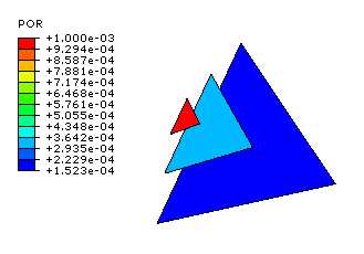
This model simulates the response of a sphere in breathing mode (a uniform radial expansion/compression mode). The model consists of one triangular ACIN3D3 element. Each node of the element is placed on a coordinate axis at a distance of 1.0 from the origin that serves as the reference point for the infinite element. The acoustic material properties do not have physical significance; the values used are for convenience only. The loading consists of applying an in-phase pressure boundary condition to all the nodes. Under this loading and geometry, the model behaves as a spherical source (an acoustic monopole) radiating in the radial direction only. The acoustic pressure, , and the acoustic far-field pressure, , at a distance from the center of the sphere are
and
where is the known acoustic pressure at some reference distance and is the wave number.
For this single-element example, you should enter a value of 1.0 for the speed of sound; thus, , where is the frequency in Hz. in this model is 1, and is 0.001. The equations for the acoustic pressure, , and the acoustic far-field pressure, , reduce to
and