Obtaining linearized stress results | ||||
|
| |||
Locate the stress linearization options.
From the main menu bar, select or click the
 tool in the
Query toolbar.
tool in the
Query toolbar.
The Query dialog box appears.
Select the endpoints for the stress line by selecting nodes or points in space or by selecting a saved path.
- Manual
-
This is the default method. You can select nodes directly from the viewport or type in node labels or points in space.
- To select nodes directly from the viewport:
-
Click
 to the right of the Start and
End fields, and click on the desired nodes in the
viewport.
to the right of the Start and
End fields, and click on the desired nodes in the
viewport.
The node labels, including the part instance name, will appear in the text field for the Start and End points of the stress line.
- To type in node labels or points in space:
-
-
In the Start text field, enter a part instance name and node label or the coordinates of a point in space. The part instance name and node label must be of the form Instance.Node; specify coordinate values as X-, Y-, and Z-coordinates separated by spaces or commas.
If you do not know the part instance names in the model, use the previous method to select a node directly from the viewport. Alternatively, you can select or click the
tool in the
Query toolbar
and choose the Probe values method to determine the
instance name and node label (for more information, see
Understanding probing).
-
Repeat the preceding step to complete the End text field.
-
- From a path
-
Toggle on From a path, and select a path name from the list that appears; you cannot use an edge list path to define the endpoints of a stress line. (For more information on paths, see Viewing results along a path.”)
Abaqus/CAE uses the endpoints of the saved path as the endpoints of the stress line. The points are defined in the same manner as they were originally defined in the path—a node list path provides node points on the model, and a point list path or circular list path provides the coordinates of points in space.
Regardless of the method you use to select the endpoints, Abaqus highlights the stress line in the viewport and labels the start and end. If you selected node points or a node list path to define the endpoints of the stress line, the labels in the viewport indicate the node numbers.
Note:
If you chose to save the stress line as a path in Step 5, Abaqus/CAE always saves a point list path—even if you selected nodes, node labels, or a node list path to define the stress line.
By default, Abaqus/CAE writes the linearized stress values (including all available components of stress and the computed linearized stress invariants) to a file called linearStress.rpt. If you do not wish to write this report, you can toggle off Write to file in the Report area of the dialog box.
You can specify a new name for the report file by entering the name in the File name field or clicking
 and choosing from the list of existing files that appears.
If you write the report to an existing file, the new data will be appended to the file by default; if you wish to overwrite the file, toggle off Append to file.
Click .
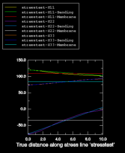
An X–Y plot similar to the one shown in Figure 1 appears in the viewport.
Figure 1. Stress linearization results.