Understanding symbol location and direction

The placement of symbols on a model can depend on the type of prescribed condition that the symbols represent and the type of region to which the prescribed condition is applied. Table 1 indicates where symbols appear on geometric models, and Table 2 indicates where symbols appear on meshed models.

Table 1. Symbol location on geometry.
Region type to which the prescribed condition is applied Location of symbols on the model
Vertex At the vertex
Edge Equally spaced along the edge
Assembly-level wire At the midpoint of the wire
Face Equally spaced over the interior of the face for directional prescribed conditions (e.g., pressure load)
  Equally spaced along the edges of the face for nondirectional prescribed conditions (e.g., surface charge and boundary conditions) 
Cell Equally spaced along each edge of the cell
Whole model At the point required to define the rigid body motion (inertia relief load only); otherwise, at the triad indicating the origin and orientation of the global coordinate system
Table 2. Symbol location on meshes.
Region type to which the prescribed condition is applied Location of symbols on the model
Node At the node
Element edge (for two-dimensional meshes) At the midpoint of the element edge
Element face (for three-dimensional meshes) At the centroid of the element face
Assembly-level wire At the midpoint of the wire
For example, Figure 1 shows a concentrated force applied to two vertices and a boundary condition applied to a surface of a geometric model.

Related Topics
Understanding symbols that represent prescribed conditions
Controlling the display of attributes
Figure 1. A concentrated force and a boundary condition.

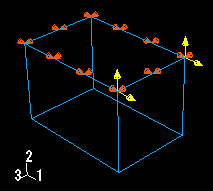
Figure 2 shows a boundary condition applied to four nodes and a pressure load applied to several element faces of a mesh.

Figure 2. A pressure load and a boundary condition.

Note:

If you apply a pressure load to a planar geometry face where the surface area is small compared to the enclosed area (such as a ring formed by two concentric circles), the load symbols may not be distributed evenly, regardless of the symbol density settings in the Assembly Display Options dialog box.

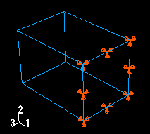
When a boundary condition fixes a degree of freedom in place, the arrow representing that component points into the region and lacks a stem. For example, the boundary condition in Figure 3 fixes degrees of freedom 1, 2, and 3 in place.

Figure 3. A boundary condition fixing degrees of freedom in place.

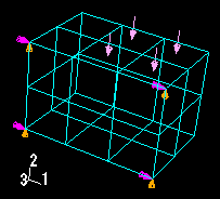
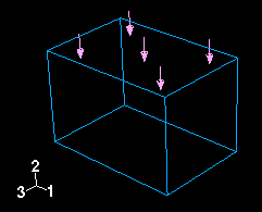
Likewise, if a positive pressure load or an Eulerian inflow boundary condition is applied to a region, the arrows representing that pressure load or boundary condition point into the region, as illustrated in Figure 4.

Figure 4. A positive pressure load.

If a load is defined to have a complex magnitude and the real and imaginary parts have different signs (for example, 2-3i), the load will appear as an arrow with two ends. Similarly, an Eulerian boundary condition that includes both inflow and outflow components will appear as an arrow with two ends.

In all other cases, arrows representing components of a prescribed condition point out from the region.

Note:

When a component of a concentrated force is zero, no arrow appears for that component. Likewise, when a boundary condition leaves a degree of freedom unconstrained, no arrow appears for that component.