Evaluating discrete fields | ||
| ||
If an element or node is found in both the region selected for the prescribed condition and the discrete field, Abaqus/CAE multiplies the magnitude of the prescribed condition by the value at each element or node to determine the final values that are submitted to the analysis. A material assignment predefined field is the only exception; this prescribed condition has no magnitude.
If an element or node is found in the region selected for the prescribed condition but not in the discrete field, the magnitude of the prescribed condition is multiplied by the default value and submitted to the analysis.
Table 1 summarizes how the value written to the input file is determined for scalar discrete fields.
| Element or node in region selected for prescribed condition? | Element or node in discrete field? | Value written to input file |
|---|---|---|
| Yes | Yes | Magnitude of prescribed condition × magnitude specified in discrete field |
| Yes | No | Magnitude of prescribed condition × default value specified in discrete field |
| No | Yes | Not written to input file |
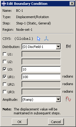
For prescribed conditions that have multiple degrees of freedom, such as displacements, prescribed condition discrete fields are used; and evaluating the discrete field becomes more complex. For prescribed conditions where you can activate the individual degrees of freedom, only the active degrees of freedom in the prescribed condition are considered; any degree of freedom that is not active in the prescribed condition will be ignored. The magnitudes specified for each degree of freedom in the prescribed condition are multiplied by either the magnitude specified in the discrete field or the default value for that degree of freedom in the discrete field.
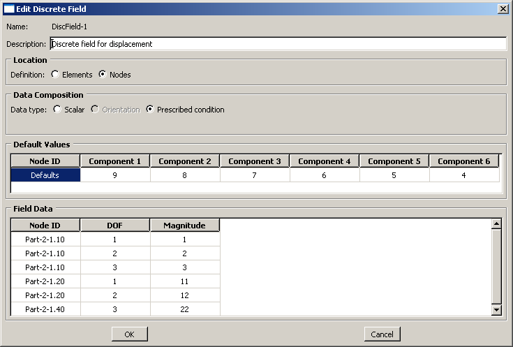
For example, if you define a displacement boundary condition, as shown in Figure 1, for Node-set-1 (containing nodes Part-2–1.10, Part-2–1.20, and Part-2–1.30) and a prescribed condition discrete field, as shown in Figure 2, the values that are submitted to the input file are shown in Table 2.
| Node ID | Degree of freedom | Value written to input file |
|---|---|---|
| Part-2-1.10 | 3 (U3) | 30 |
| Part-2-1.10 | 4 (UR1) | 600 |
| Part-2-1.20 | 3 (U3) | 70 |
| Part-2-1.20 | 4 (UR1) | 600 |
| Part-2-1.30 | 3 (U3) | 70 |
| Part-2-1.30 | 4 (UR1) | 600 |
| Part-2-1.40 | 3 (U3) | None |
Degrees of freedom for boundary conditions and predefined fields that result in a zero magnitude are written to the input file as such; however, degrees of freedom for loads that result in zero magnitudes are not written to the input file.
When creating discrete fields that will be used with assembly-level and history objects, such as loads or interactions, you must specify the complete name of the node or element numbers, as described in Naming conventions.