Slender pipe subject to drag: the “reed in the wind” | ||
| ||
ProductsAbaqus/StandardAbaqus/Aqua
Currents flowing past a pipeline result in drag loading, which must be accounted for in designing restraints and moorings for the pipeline. Drag loadings vary approximately as the square of the relative normal velocity (difference between pipe and fluid velocities), and effects can be dramatic, as illustrated in the present example. Numerically drag loading results in an unsymmetric load stiffness contribution, so the resulting finite element equations are also unsymmetric.
The equation of Morison et al. (1950) is used in Abaqus to account for drag loading. The total drag force is divided into tangential, transverse, inertia, and lift contributions. The first two of these relate the drag force to the square of relative velocity, through the experimentally determined tangential and transverse drag coefficients, respectively. The inertia drag force is an “added mass” contribution based on the relative acceleration. The lift term is relevant when the pipeline lies on the seafloor or near a platform, so that the current velocity varies across the pipe. For details of Morison's drag formulation, see Drag, inertia, and buoyancy loading.
Problem description
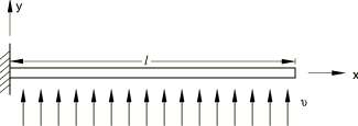
A pipe 304.8 m (1000 ft) long, initially straight and stress-free, is loaded by a uniform cross-current of 0.762 m/s (2.5 ft/sec) as shown in Figure 1. The outside radius of the pipe is 76.2 mm (0.25 ft), and its wall thickness is 15.24 mm (0.05 ft), so the pipe is “slender” and virtually inextensible (its extensional stiffness is much greater than its flexural stiffness). Abaqus provides a family of two-dimensional and three-dimensional hybrid beam elements designed specifically for use in such cases. In this case five B23H elements are used to model the pipeline.
The pipe is made of a linear elastic material, with a Young's modulus of 206.8 GPa (4.32 × 10⁹ lb/ft2). A general beam section is used for the pipe section specification. This choice avoids numerical integration of the pipe section during the analysis and, hence, reduces computer costs. Numerical integration over the beam section would be necessary if plasticity or other material nonlinearities were to be considered.
The loading on the pipe results from a uniform current flowing in the global y-direction, as shown in Figure 1. The current velocity is 0.762 m/s (2.5 ft/s), and the density of the water is 1000 kg/m3 (1.94 slug/ft3). The transverse drag coefficient is 1.2, and the tangential drag coefficient is 0.002. The large difference between these coefficients reflects the different effects transverse and tangential flow have on the pipeline, the tangential drag being primarily a skin friction effect only. The pipeline is assumed to be built-in at one end, as shown in Figure 1.
![]()
Results and discussion
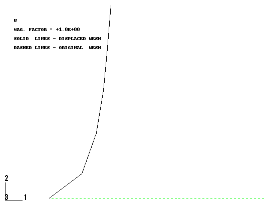
The final pipeline configuration resulting from the current induced drag loads is shown in Figure 2. The dramatic effect of the drag loads is evident. It is typical of such monotonically loaded, geometrically nonlinear problems to require smaller load increments for convergence at early stages of the analysis, and the load increments can increase as the analysis progresses. This is because the system is most flexible in its original configuration. By reducing load steps when convergence is difficult, the automatic loading option in Abaqus avoids user experimentation to obtain convergent solutions. This greatly eases the task of obtaining solutions and generally reduces the computer costs of generating such solutions. For this reason automatic incrementation is recommended for problems of this type.
![]()
References
- “The Force Exerted by Surface Waves on Piles,” Transactions, American Institute of Mining, Metallurgical and Petroleum Engineers, Inc., vol. 189, pp. 149–154, 1950.
![]()
Figures