Freezing of a square solid: the two-dimensional Stefan problem | ||
| ||
ProductsAbaqus/StandardAbaqus/Explicit
Heat conduction problems involving latent heat effects occur often in practice (examples are metal casting and permafrost meltout) but are not simple to solve. In some cases the phase change occurs with little latent heat effect and rapid temperature changes can partially suppress the change, as in the case of the amorphous/crystalline polymer phase change. For such cases Abaqus/Standard provides a user subroutine, HETVAL, in which the user can program the kinetics of the phase change and the consequent latent heat exchange in terms of solution-dependent state variables. In contrast, a liquid/solid phase change is usually fairly abrupt and is accompanied by a strong latent heat effect. This case is the one considered in this example.
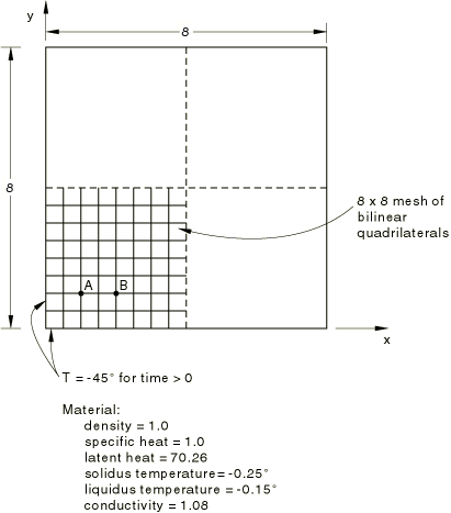
The problem is the two-dimensional Stefan problem (Figure 1): a square block of material is initially liquid, just above the freezing temperature. The temperature of its outside perimeter is reduced suddenly by a large value, so that the block starts to freeze from the outside toward the core. The freezing has a very large latent heat effect associated with it that dominates the solution. The problem has no exact solution, but a number of researchers have provided approximate solutions. Probably the most accurate of these is the numerical solution of Lazaridis (1970), who considers the problem as a moving boundary condition problem. Lazaridis's solution is used here as verification of the Abaqus modeling of such cases.
Problem description
The block is a square of dimension 8 × 8 length units. Because of symmetry we need to consider only an octant, but we model a quarter for simplicity in generating the mesh.
Severe latent heat effects involve moving boundary conditions (the freezing front), across which the spatial gradient of temperature, , is discontinuous. Simple finite elements, such as the linear and quadratic elements used in Abaqus, do not allow gradient discontinuities within an element, although they do allow such discontinuities between elements in the direction of the normal to their sides. Since the actual problem involves discontinuities along surfaces moving through the mesh, the best we can do with a fixed grid of simple elements is to use a fine mesh of lowest-order elements, thus providing a high number of gradient discontinuity surfaces. In Abaqus/Standard two-dimensional heat transfer elements (DS3 and DS4) and first-order coupled temperature-displacement elements (CPE4T and CPEG4T) are used to model the plate. The meshes used are coarse for the problem; but they suffice to give reasonable solutions and, thus, verify the capability. In practical cases a more refined model is recommended. In Abaqus/Explicit two- and three-dimensional, first-order coupled temperature-displacement elements (CPE4RT, C3D8RT, and SC8RT) are used to model the plate.
![]()
Material
The material properties (in consistent units) are
| Density | 1.0 |
| Specific heat | 1.0 |
| Latent heat of freezing | 70.26 |
| Freezing temperature | 0° |
| Thermal conductivity | 1.08 |
This set of values includes a latent heat effect that is far more severe than that in any material of practical importance. This value is deliberately chosen to provide a stringent test of the accuracy of the algorithm.
The latent heat must be specified in Abaqus over a temperature range. For this purpose we give the solidus and liquidus temperatures as −0.25° and −0.15°, respectively.
In the simulations involving Abaqus/Explicit dummy mechanical properties are used to complete the material definition.
![]()
Boundary conditions
The symmetry lines are insulated; this is the default surface boundary condition and, so, need not be specified. The outside surfaces must be reduced at time zero to −45°. This value can be specified directly; however, we ramp the temperature down to −45° over a time of 0.05 to prevent the automatic time incrementation scheme in Abaqus/Standard from choosing very small time increments at the beginning of the simulation.
![]()
Time increment controls
Automatic time incrementation is chosen, which is the usual option for transient heat conduction problems. In Abaqus/Standard a maximum temperature change of 4° is allowed per time increment to allow the time increment to increase to large values at later times as the solution smoothes out.
![]()
Results and discussion
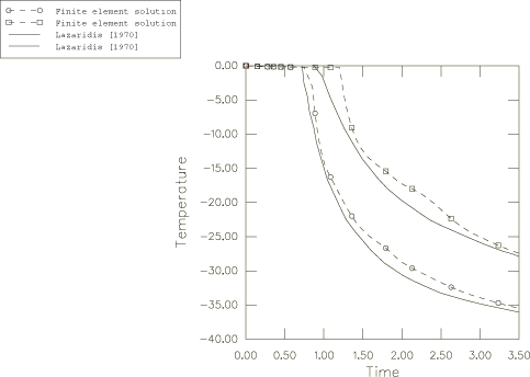
Temperature-time plots for points A and B of Figure 1 are shown in Figure 2, where they are compared to Lazaridis's (1970) numerical solution. The numerical results shown in this figure are based on the solution obtained with Abaqus/Standard. The Abaqus results are quite accurate considering the coarseness of the mesh used and the extreme severity of the latent heat effect in this example. The solution oscillates about Lazaridis's results because the finite element mesh allows temperature gradient discontinuities only at element boundaries, so that the fusion fronts effectively jump between these locations. This effect is also the reason for the delay in the start of the temperature drop.
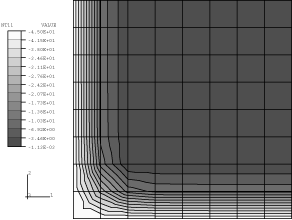
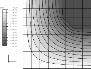
Figure 3 and Figure 4 show isotherm contour plots at different times. The form of the solution is very clear from these plots.
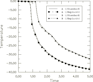
The results obtained with Abaqus/Explicit compare well with those obtained with Abaqus/Standard, as illustrated in Figure 5. This figure compares the results obtained with Abaqus/Explicit for the temperature history of points A and B against the same results obtained with Abaqus/Standard.
![]()
Input files
Abaqus/Standard input files
- freezingofsolid_2d.inp
-
Input data for the two-dimensional problem.
- freezingofsolid_3d.inp
-
Similar model in three dimensions.
- freezingofsolid_postoutput.inp
-
POST OUTPUT analysis.
- freezingofsolid_2d_usr_umatht.inp
-
Two-dimensional simulation of the problem with the material behavior defined in user subroutine UMATHT to illustrate the coding of this subroutine.
- freezingofsolid_2d_usr_umatht.f
-
User subroutine UMATHT used in freezingofsolid_2d_usr_umatht.inp.
- freezingofsolid_ds3.inp
-
Two-dimensional analysis with DS3 elements.
- freezingofsolid_ds4.inp
-
Two-dimensional analysis with DS4 elements.
- freezingofsolid_deftorigid.inp
-
Two-dimensional analysis with CPE4T elements declared as rigid.
- freezingofsolid_cpeg4t.inp
-
Two-dimensional analysis with CPEG4T elements.
Abaqus/Explicit input files
- freezingofsolid_xpl_cpe4rt.inp
-
Two-dimensional analysis with CPE4RT elements.
- freezingofsolid_xpl_c3d8rt.inp
-
Three-dimensional analysis with C3D8RT elements.
- freezingofsolid_xpl_sc8rt.inp
-
Three-dimensional analysis with SC8RT elements.
![]()
References
- “A Numerical Solution of the Multidimensional Solidification (or Melting) Problem,” International Journal of Heat and Mass Transfer, vol. 13, 1970.
![]()
Figures