Fitting of elastomeric foam test data

This example illustrates the use of uniaxial compression data or uniaxial compression and simple shear data to fit the hyperfoam constants in the hyperelastic foam model.

The following topics are discussed:

Problem description
Fitting procedure
Results and discussion
Input files
References
Figures

ProductsAbaqus/Standard

Elastomeric foams are cellular materials that have the following primary mechanical characteristics:

They can deform elastically up to 90% compression. This is their dominant mode of deformation.
Their porosity permits very large volumetric deformations. This is in contrast to solid rubbers that are approximately incompressible.

Examples of elastomeric foam materials are cellular polymers such as cushions, padding, and packaging materials. Foams are often used for their excellent energy absorption properties—for a certain stress level, the energy absorbed by foams is substantially greater than by ordinary stiff elastic materials.

Another class of foam materials are the crushable foams that can undergo permanent (plastic) deformations. These materials are modeled using the crushable foam material model.

Elastomeric foam materials are modeled using the hyperelastic foam model (Hyperelastic behavior in elastomeric foams), which is a nonlinear elastic model. The elastic behavior of the foams is based on the strain energy function

U = \underset{i = 1}{\sum^{N}} \frac{2 μ_{i}}{α_{i}^{2}} [{\hat{λ}}_{1}^{α_{i}} + {\hat{λ}}_{2}^{α_{i}} + {\hat{λ}}_{3}^{α_{i}} - 3 + \frac{1}{β_{i}} (J_{e ℓ}^{- α_{i} β_{i}} - 1)],

where

{\hat{λ}}_{i} = J_{t h}^{- \frac{1}{3}} λ_{i} \to {\hat{λ}}_{1} {\hat{λ}}_{2} {\hat{λ}}_{3} = J_{e ℓ}

and $λ_{i}$ are the principal stretches. The elastic and thermal volume ratios, $J_{e ℓ}$ and $J_{t h},$ are

J_{e ℓ} = \frac{J}{J_{t h}} and J_{t h} = {(1 + ε_{t h})}^{3},

where J is the total volume ratio (current volume divided by original volume), and the thermal strain $ε_{t h}$ follows from the temperature and the isotropic thermal expansion coefficient defined in the thermal expansion material property. Time- or frequency-dependent elastic behavior is modeled through viscoelastic behavior.

The coefficients, $μ_{i}$ , are related to the initial shear modulus, $μ_{0}$ ,

μ_{0} = \underset{i = 1}{\sum^{N}} μ_{i};

the initial bulk modulus, $K_{0}$ , follows from

K_{0} = \underset{i = 1}{\sum^{N}} 2 μ_{i} (\frac{1}{3} + β_{i});

and $β_{i}$ is related to Poisson's ratio $ν_{i}$ ,

β_{i} = \frac{ν_{i}}{1 - 2 ν_{i}} .

This example shows how to derive the hyperfoam constants $μ_{i}$ , $α_{i}$ , and $β_{i}$ from a set of material test data.

Problem description

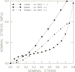
For this example the test data are composed of uniaxial compression and simple shear data whose nominal stress–nominal strain curves are shown in Figure 1. The uniaxial compression curve (labeled “1” in the figure) can be broken down into three stages:

At small strains ( $<$ 5%) the foam deforms in a linear, elastic way due to cell wall bending.
This is followed by a plateau of deformation with a relatively small range of stress caused by the elastic buckling of the cell walls.
At higher strains a region of densification occurs where the cell walls crush together resulting in a rapid increase of compressive stress.

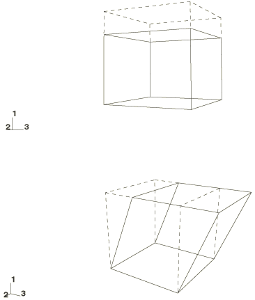
For this material the effective Poisson's ratio is zero, which is evident by the absence of lateral displacements, as seen in Figure 2 in which a single continuum element illustrates the two deformation modes: uniaxial compression and simple shear.

The simple shear deformation results in a combination of compression and tension of the cell walls. In addition to the shear stress (labeled “2” in Figure 1), a transverse tensile stress (labeled “3” in the figure) is developed normal to the shear direction—this is called the Poynting effect. This transverse stress is included in the test data in addition to the shear stress.

Fitting procedure

In Abaqus the test data are specified as nominal stress–nominal strain data pairs using combinations of uniaxial test data, biaxial test data, simple shear test data, planar test data, and volumetric test data for hyperelastic foam with material constants computed by Abaqus from the test data. In addition, the effective Poisson's ratio can be specified for the hyperelastic foam.

For each stress-strain data pair, Abaqus generates an expression for the stress in terms of the stretches and the unknown hyperfoam constants. For the uniaxial, equibiaxial, planar, and volumetric deformation cases, the nominal stress $T_{C}$ is

T_{C} = \frac{\partial U}{\partial λ_{C}} = \frac{2}{λ_{C}} \overset{N}{\sum_{i = 1}} \frac{μ_{i}}{α_{i}} [λ_{C}^{α_{i}} - J_{e ℓ}^{- α_{i} β_{i}}],

where U is the strain energy potential and $λ_{C}$ is the stretch in the primary displacement direction.

For the simple shear case, the nominal shear stress $T_{S}$ is

T_{S} = \frac{\partial U}{\partial γ} = \overset{2}{\sum_{j = 1}} [\frac{2 γ}{2 (λ_{j}^{2} - 1) - γ^{2}} \overset{N}{\sum_{i = 1}} \frac{μ_{i}}{α_{i}} (λ_{j}^{α_{i}} - 1)],

where $γ$ is the shear strain and $λ_{j}$ are the two principal stretches in the plane of shearing and are related to the shear strain by

λ_{1, 2} = \sqrt{1 + \frac{γ^{2}}{2} \pm γ \sqrt{1 + \frac{γ^{2}}{4}}} .

For the n stress-strain pairs the following error measure E is minimized:

E = \overset{n}{\sum_{i = 1}} {(1 - T_{i}^{th} / T_{i}^{test})}^{2},

where $T_{i}^{test}$ is a stress value from the test data and $T_{i}^{th}$ is one of the stress expressions described above.

As the energy potential is a nonlinear function of $α_{i}$ and $β_{i}$ , a nonlinear least squares procedure similar to that of Twizell and Ogden (1983) is used in Abaqus to determine $μ_{i}, α_{i}$ , and $β_{i}$ simultaneously. If the POISSON parameter is specified as the effective Poisson's ratio $ν$ , then all the $β_{i}$ constants are directly computed as

β_{i} = \frac{ν}{1 - 2 ν} .

After a set of material constants is obtained, Abaqus performs material stability checks along the primary deformation modes using the Drucker stability criterion:

d τ : d ε > 0 ⟹ d ε \cdot D : d ε > 0,

where $d τ$ is the Kirchhoff stress increment due to the logarithmic strain increment, $d ε$ , and $D$ is the tangential material stiffness. For the stability criterion to be satisfied, $D$ must be positive-definite. The analysis input file processor will give warning messages if $D$ loses its positive-definite property, thereby defining strain states that are likely to result in unstable material behavior. The deformation modes examined are uniaxial, equibiaxial, planar, and volumetric deformation in tension and compression and the simple shear mode.

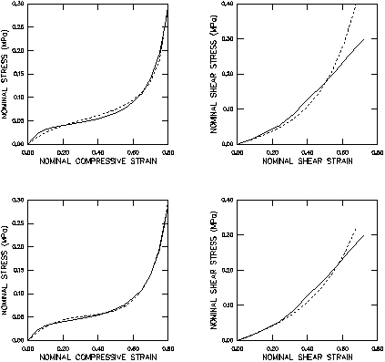
Fitting case 1—results using uniaxial compression and simple shear data

Both types of test data are used in fitting the hyperfoam constants for order $N =$ 2 (with four constants: $μ_{1}, α_{1}, μ_{2}, α_{2}$ ; the $β_{1}, β_{2}$ constants are zero since the effective Poisson's ratio is zero) and order $N =$ 3 (with six constants). Both the shear stress and the transverse tensile stress are used for the simple shear data. The $N =$ 3 parameters fail the Drucker stability test for five deformation modes, while the $N =$ 2 parameters predict no instability at all.

A single 8-node continuum element C3D8R of unit dimensions is subjected to enforced boundary conditions simulating the two deformation modes as shown in Figure 2. Since Abaqus outputs true (Cauchy) stress and logarithmic strain, a method of deriving nominal stress–nominal strain results is described in the listings of the data files at the end of this example.

The fits as shown in Figure 3 for both values of N are accurate up to the maximum strain of 80% for the uniaxial compression case. For the simple shear case the fit is accurate up to shear strains of about 50%; beyond that, the Abaqus shear results stiffen up faster than the shear test data.

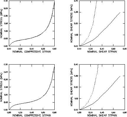
Fitting case 2—results using uniaxial compression data only

Commonly only one type of test data may be available to the user. For this example the consequences of fitting the hyperfoam constants using only the uniaxial compression data are examined. Both $N =$ 2 and $N =$ 3 parameters pass all the Drucker stability tests. Figure 4 shows the results of the two deformation modes in contrast with fitting case 1.

The uniaxial compression results for both values of N match the test data extremely well, as expected since the hyperfoam constants are fit using only the uniaxial data. However, in the simple shear case considerable disparities are seen between the numerical and test data at the onset of finite strains—the shear results of fitting case 1 are definitely superior.

Results and discussion

For these test data the $N =$ 2 model seems adequate in providing close correlations (it is stable, where the $N =$ 3 model is not). However, this example also illustrates that the shear behavior is not satisfactorily reproduced when only uniaxial test data are used in fitting the hyperfoam constants. The inadequacy can be attributed to the fact that, in simple shear, certain directions are in tension. This tension behavior cannot be characterized properly with compression data only. This observation is similar to the one made for incompressible hyperelastic materials, where there is no guarantee that other deformation modes besides the test data modes can be reproduced to an acceptable accuracy.

However, for hyperelastic foams the ample compressibility reduces the different axial deformation modes (e.g., biaxial, triaxial, etc.) into a “superposition” of several uniaxial states at different orientations. This is particularly true for compression states, where buckling of cell walls under loading in one direction is quite independent from that in perpendicular directions. Thus, it is not uncommon that a single uniaxial compression test may be sufficient to characterize the material behavior if the application is compression dominated. However, it is preferable to use test data derived from different deformation modes.

Input files

foamdatafitting_compress.inp: Uniaxial compression mode.
foamdatafitting_shear.inp: Simple shear deformation mode.

Change the value of the parameter N of the HYPERFOAM option to use a different order of the strain energy function. Remove the simple shear stress-strain data from the material definition to run the cases of using uniaxial compression data only.

References

Twizell, E. H., and R. W. Ogden, “Non-Linear Optimization of the Material Constants in Ogden's Stress-Deformation Function for Incompressible Isotropic Elastic Materials,” J. Austral. Math. Soc. Ser. B, vol. 24, pp. 424–434, 1983.

Figures

Figure 1. Uniaxial compression and simple shear test data.

Figure 2. Uniaxial compression and simple shear deformation modes.

Figure 3. Results using uniaxial compression and simple shear data. Solid line: experimental data. Dashed line: Abaqus results.

Figure 4. Results using uniaxial compression data only. Solid line: experimental data. Dashed line: Abaqus results.