Composite shells in cylindrical bending

This example verifies the transverse shear stress calculations in Abaqus for multilayer composite shells and demonstrates the use of the plane stress orthotropic failure measures. A discussion of the transverse shear stresses obtained by composite solids in Abaqus/Standard is included in this example. The problem consists of a two- or three-layer plate subjected to a sinusoidal distributed load, as described by Pagano (1969). The resulting transverse shear and axial stresses through the thickness of the plate are compared to two existing analytical solutions by Pagano (1969). The first solution is derived from classical laminated plate theory (CPT), while the second is an exact solution from linear elasticity theory.

The following topics are discussed:

Problem description
Failure measures
Results and discussion
Input files
References
Figures

ProductsAbaqus/StandardAbaqus/Explicit

Problem description

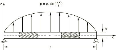
A schematic of the model is shown in Figure 1. The structure is a composite plate composed of orthotropic layers of equal thickness. It is simply supported at its ends and bounded along its edges to impose plane strain conditions in the y-direction. Each layer models a fiber/matrix composite with the following properties:

$E_{L}$	172.4 GPa (25 × 10⁶ lb/in²)
$E_{T}$	6.90 GPa (1.0 × 10⁶ lb/in²)
$G_{L T}$	3.45 GPa (0.5 × 10⁶ lb/in²)
$G_{T T}$	1.38 GPa (0.2 × 10⁶ lb/in²)
$ν_{L T} = ν_{T T}$	0.25

where L signifies the direction parallel to the fibers and T signifies the transverse direction. In Abaqus/Standard two methods are used to specify the lay-up definition for the conventional shell element model. First, a composite shell section is defined to specify the thickness, number of integration points, material name, and orientation of each layer. Second, a composite general shell section is defined to specify the thickness, material name, and angle of orientation relative to the section orientation (the default shell directions in this case) for each layer. In Abaqus/Explicit only the former method is used. The material properties are specified using the orthotropic elastic in plane stress definition. The orientation of the fibers in each layer is defined by an in-plane rotation angle measured relative to the local shell directions or relative to an orientation definition given for the general shell section.

In addition to the methods outlined above, a third method of stacking continuum shell elements is used to specify the lay-up definition for a composite model. This method can be used effectively to study localized behavior, since continuum shell elements handle high aspect ratios between the in-plane dimension and the thickness dimension well.

The lay-up definition for the continuum (solid) element model in Abaqus/Standard is specified using a composite solid section definition. The thickness, material name, and orientation definition are specified for each layer.

A distributed load with a sinusoidal distribution in space, $p = p_{0} \sin (π x / l)$ , is applied to the top of the composite plate. In Abaqus/Standard the load is applied using user subroutine DLOAD in a static linear analysis step. In addition, an Abaqus/Standard input file is included that demonstrates the use of the DCOUP3D element to apply this distributed load. In Abaqus/Explicit the load is applied instantaneously at time $t =$ 0.

Two composite plates are analyzed in this example. The first is a two-layer plate with the fibers oriented parallel and orthogonal to the x-axis in the bottom and top layer, respectively. In the second plate, which has three layers of equal thickness, the fibers in the outer layers are oriented parallel to the x-axis, while the fibers in the middle layer are orthogonal to the x-axis. The span-to-thickness ratio of the plates, $s = l / h$ , is varied from 4 to 30 in the Abaqus/Standard analysis; in Abaqus/Explicit this ratio is 4 throughout the analysis.

A 1 × 10 mesh of second-order S8R shell elements is used to model the plates in Abaqus/Standard. A 2 × 10 mesh of first-order S4R shell elements is used to model the plates in Abaqus/Explicit. The S4R, S8R, and S8RT shell elements are well-suited for modeling thick composite shells since they account for transverse shear flexibility. Five integration points are specified through the thickness of each layer with the models that use the shell section. This provides sufficient data to describe the stress distributions through the thickness of each layer. For the models that use the general shell section, only three points are available for output. (Since the analysis is linear elastic, three points are sufficient to determine all fields through the thickness.) The plate with the lowest span-to-thickness ratio is also analyzed with Abaqus/Standard using a 1 × 10 mesh of second-order C3D20R composite solid elements.

To illustrate the stacking capability of continuum shell elements, several meshes are provided for the two- and three-layer plates with a span-to-thickness ratio of 4. The two-layer plate is modeled with a 2 × 10 mesh of SC8R elements, each element representing a single layer of the 90/0 composite plate. One model of the three-layer plate uses a 1 × 10 mesh of SC8R elements using a single element through the thickness with a composite section definition. Another model of the three-layer plate uses a 3 × 10 mesh of SC8R elements, each element representing a single layer of the 0/90/0 composite plate. Additional models of the three-layer plate with 6, 12, and 24 elements through the thickness are provided. In these models each composite layer is modeled with 2, 4, and 8 elements through the thickness, respectively.

Additional input files using SC8R elements are included to illustrate defining the stacking and thickness direction independent of the element nodal connectivity.

Failure measures

The plane stress orthotropic failure measures are defined in Plane stress orthotropic failure measures. To demonstrate their use, let the limit stresses and limit strains be given as follows:

Stress Values:	$X_{t}$	$X_{c}$	$Y_{t}$	$Y_{c}$	S
(GPa)	2.07 × 10⁻⁴	−8.28 × 10⁻⁵	3.45 × 10⁻⁶	−1.03 × 10⁻⁵	6.89 × 10⁻⁶
(lb/in²)	30.0	−12.0	0.5	−1.5	1.0
Strain Values:	$X_{ϵ}_{t}$	$X_{ϵ}_{c}$	$Y_{ϵ}_{t}$	$Y_{ϵ}_{c}$	$S_{ϵ}$
	17. × 10⁻²	−7. × 10⁻²	5. × 10⁻²	−1.3 × 10⁻²	11. × 10⁻²

The scaling factor for the Tsai-Wu coefficient $F_{12}$ is $\overset{*}{f} =$ 0.0. These values are chosen such that failure occurs under the stress-based failure criteria for the given loading in the two-layer case with $s =$ 4.

Results and discussion

The results for each of the analyses are discussed in the following sections.

Abaqus/Standard results

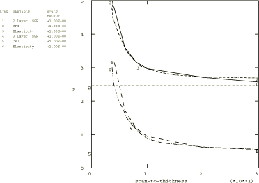
Figure 2 shows the maximum z-displacement as a function of the span-to-thickness ratio of the two- and three-layer plates in a normalized form as

w = \frac{100 E_{T} h^{3} u_{z} (l / 2)}{l^{4}} .

As seen in the figure, the finite element displacements for both the two- and three-layer plates agree well with the prediction from elasticity theory for a wide range of s values. The CPT results are stiff at low values of s since shear flexibility is neglected.

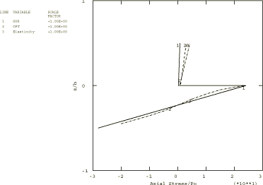
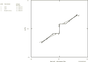
For $s =$ 4, Figure 3 and Figure 4 show the transverse shear stress (TSHR13) and the axial stress (S11) distributions through the plate thickness for the two-layer plate normalized as

{\bar{τ}}_{x z} = \frac{τ_{x z} (0, z)}{p_{o}}

and

{\bar{σ}}_{x} = \frac{σ_{x} (l / 2, z)}{p_{o}} .

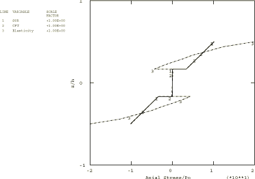
Figure 5 and Figure 6 show the corresponding results for the three-layer plate. It is seen that the shell element results are much closer to the predictions of CPT than to elasticity theory because of the assumption of linear stress variation through the thickness in the first-order shear flexible theory used for elements such as S8R and S4R.

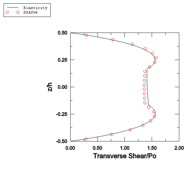
Figure 7 compares the elasticity solution of the transverse shear distribution for the three-layer plate to an approximate solution using the output variable SSAVG4. SSAVG4 is the average transverse shear stress in the local 1-direction. Since SSAVG4 is constant over an element, mesh refinement (in this case 24 continuum shell elements through the thickness) is typically required to capture the variation of shear stress through the thickness of the plate.

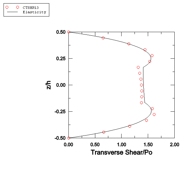
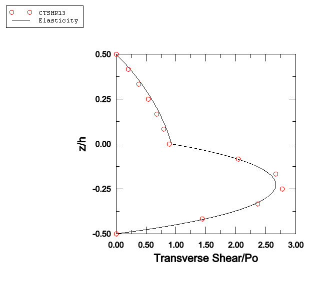
The output variables CTSHR13 and CTSHR23 offer a more economical alternative to SSAVG4 and SSAVG5 for estimating shear stress in stacked continuum shells. Figure 8 and Figure 9 show very good agreement between the elasticity solution of the transverse shear distribution for the three- and two-layer plates to the solution using the output variable CTSHR13 for a 3 × 10 and 2 × 10 mesh of continuum shell elements, respectively. The shear stress computed using CTSHR13 is continuous across the continuum shell element interfaces. In addition, while the estimates of the transverse shear distributions using SSAVG4 and CTSHR13 (shown in Figure 7 and Figure 8) are both good, using CTSHR13 requires a mesh of only 3 continuum shell elements through the thickness, as compared to 24 elements for SSAVG4.

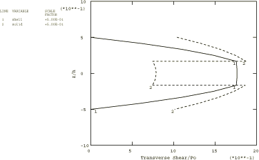
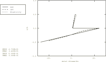
Figure 10 compares the transverse shear stress distribution obtained with the solid element model with the shell element result. The figure shows that the transverse shear stresses predicted by solid elements do not vanish at the free surfaces of the structure. It also shows that the stress is discontinuous at layer interfaces. The reason for this is that in the composite solid element, the transverse shear stresses are obtained directly from the displacement field in contrast to the shell element, where the transverse shear stresses are obtained from an equilibrium calculation. These deficiencies decrease if the number of solid elements used in the discretization through the section thickness is increased. Although the transverse shear stresses are inaccurate, the displacement field and components of stress in the plane of the layer (not shown here) are in much better agreement with the analytical result. In fact, these results are somewhat better than the results obtained with the S8R elements. The composite solid elements were not used to analyze the thinner plates since the solid elements would not have any advantage over plate elements in that case.

For $s =$ 10, Figure 11 and Figure 12 show that the transverse shear and axial stress distributions of the finite element results—along with the CPT predictions—agree with elasticity theory. The stress distributions become more accurate with increasing span-to-thickness ratio (as the plate becomes thinner in comparison to the span).

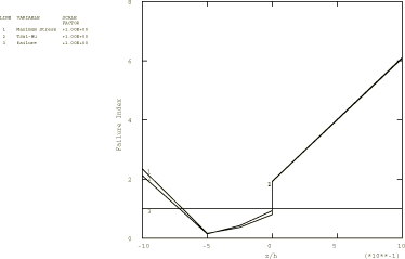
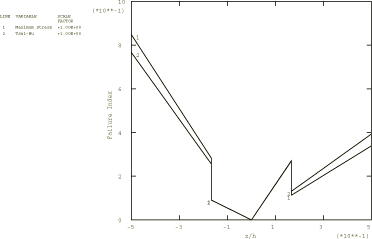
In Figure 13 and Figure 14 the maximum stress theory and Tsai-Wu theory failure indices are plotted as a function of the normalized distance from the midsurface for the two- and three-layer cases, respectively. The indices are calculated at the center of the plate for S8R elements with $s =$ 4. Values of the failure index greater than or equal to 1.0 indicate failure. Discontinuous jumps in the failure index occur at layer boundaries as a result of the orientation of the material. The strain levels are well below those required for failure, so no strain-based failure indices are plotted.

Abaqus/Explicit results

The explicit dynamic analysis is run for a sufficiently long time so that a quasi-static state is reached—that is, the plates are in steady-state vibration. Since step loadings are applied, static solutions of stresses can be obtained as half of their vibration amplitudes.

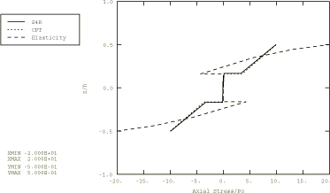
Figure 15 and Figure 16 show the transverse shear stress (TSHR13) and the axial stress (S11) distributions through the plate thickness for the two-layer S4R model normalized as:

{\bar{τ}}_{x z} = \frac{τ_{x z} (0, z)}{p_{o}}

and

{\bar{σ}}_{x} = \frac{σ_{x} (l / 2, z)}{p_{o}},

compared with classical plate theory (CPT) and linear elasticity theory.

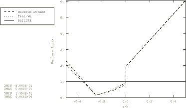
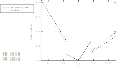
Figure 17 and Figure 18 show the corresponding results for the three-layer plate. In Figure 19 and Figure 20, the maximum stress theory and Tsai-Wu theory failure indices are plotted as a function of the normalized distance from the midsurface for the two- and three-layer cases, respectively. The indices are calculated at the center of the plate. Values of the failure index greater than or equal to 1.0 indicate failure. Discontinuous jumps in the failure index occur at layer boundaries due to the orientation of the material. The strain levels are well below those required for failure, so no strain-based failure indices are plotted.

Input files

Abaqus/Standard input files

compositeshells_s8r.inp: Three-layer plate with $s =$ 4 using S8R elements.
compositeshells_s8r.f: User subroutine defining nonuniform distributed load for use with compositeshells_s8r.inp.
compositeshells_s8r_gensect.inp: Three-layer plate with $s =$ 4 using S8R elements and SHELL GENERAL SECTION.
compositeshells_s8r_gensect.f: User subroutine DLOAD used in compositeshells_s8r_gensect.inp.
compositeshells_s4.inp: S4 element model.
compositeshells_s4.f: User subroutine DLOAD used in compositeshells_s4.inp.
compositeshells_s4_gensect.inp: S4 element model with SHELL GENERAL SECTION.
compositeshells_s4_gensect.f: User subroutine DLOAD used in compositeshells_s4_gensect.inp.
compositeshells_s4_dcoup3d.inp: S4 element model loaded using a DCOUP3D element.
compositeshells_s4r.inp: S4R element model.
compositeshells_s4r.f: User subroutine DLOAD used in compositeshells_s4r.inp.
compositeshells_s4r_gensect.inp: S4R element model with SHELL GENERAL SECTION.
compositeshells_s4r_gensect.f: User subroutine DLOAD used in compositeshells_s4r_gensect.inp.
compositeshells_c3d20r.inp: C3D20R composite solid element model.
compositeshells_c3d20r.f: User subroutine DLOAD used in compositeshells_c3d20r.inp.
compositeshells_sc8r_stackdir_1.inp: SC8R model using STACK DIRECTION=1.
compositeshells_sc8r_stackdir_2.inp: SC8R model using STACK DIRECTION=2.
compositeshells_sc8r_stackdir_3.inp: SC8R model using STACK DIRECTION=3.
compositeshells_sc8r_gensect.inp: SC8R model using SHELL GENERAL SECTION.
compshell2_std_sc8r_stack_2.inp: Two-layer plate with SC8R elements, two elements stacked through the thickness.
compshell3_std_sc8r_stack_1.inp: Three-layer plate with SC8R elements, single element through the thickness.
compshell3_std_sc8r_stack_3.inp: Three-layer plate with SC8R elements, three elements stacked through the thickness.
compshell3gs_std_sc8r_stack_3.inp: Three-layer plate with SC8R elements, three elements stacked through the thickness using a general shell section definition.
compshell3_std_sc8r_stack_6.inp: Three-layer plate with SC8R elements, six elements stacked through the thickness.
compshell3_std_sc8r_stack_12.inp: Three-layer plate with SC8R elements, 12 elements stacked through the thickness.
compshell3_std_sc8r_stack_24.inp: Three-layer plate with SC8R elements, 24 elements stacked through the thickness.
compositeshells_sc8r.f: User subroutine DLOAD used with the SC8R models.

Abaqus/Explicit input files

compshell3_1.inp: Three-layer plate modeled with S4R elements.
compshell3_1_sc8r.inp: Three-layer plate modeled with SC8R elements.
compshell3_1_sc8r_stackdir_1.inp: Three-layer plate modeled with SC8R elements using STACK DIRECTION=1.
compshell3_1_sc8r_stackdir_2.inp: Three-layer plate modeled with SC8R elements using STACK DIRECTION=2.
compshell3_1_sc8r_stackdir_3.inp: Three-layer plate modeled with SC8R elements using STACK DIRECTION=3.
compshell3_2.inp: Three-layer plate with a different thickness and modeled with S4R elements.
compshell2_1.inp: Two-layer plate modeled with S4R elements.
compshell2_2.inp: Two-layer plate modeled with S4R elements.
compshell2_1_sc8r.inp: Two-layer plate modeled with SC8R elements.

References

Pagano, N. J., “Exact Solutions for Composite Laminates in Cylindrical Bending,” Journal of Composite Materials, vol. 3, pp. 398–411, 1969.

Figures

Figure 1. Composite plate subject to distributed loading.

Figure 2. Maximum deflection of two- and three-layer plates with various span-to-thickness ratios; Abaqus/Standard analysis.

Figure 3. Transverse shear stress distribution through the thickness of a two-layer plate (

s =

4); Abaqus/Standard analysis.

Figure 4. Axial stress distribution through the thickness of a two-layer plate (

s =

4); Abaqus/Standard analysis.

Figure 5. Transverse shear stress distribution through the thickness of a three-layer plate (

s =

4); Abaqus/Standard analysis.

Figure 6. Axial stress distribution through the thickness of a three-layer plate (

s =

4); Abaqus/Standard analysis.

Figure 7. Comparison of the elasticity solution of the transverse shear stress distribution in a three-layer plate to the output variable SSAVG4 with 24 SC8R elements stacked through the thickness; Abaqus/Standard analysis.

Figure 8. Comparison of the elasticity solution of the transverse shear stress distribution in a three-layer plate to the output variable CTSHR13 with 3 SC8R elements stacked through the thickness; Abaqus/Standard analysis.

Figure 9. Comparison of the elasticity solution of the transverse shear stress distribution in a two-layer plate to the output variable CTSHR13 with 2 SC8R elements stacked through the thickness; Abaqus/Standard analysis.

Figure 10. Transverse shear stress distribution through the thickness of a three-layer plate (

s =

4): shells versus solid elements; Abaqus/Standard analysis.

Figure 11. Transverse shear stress distribution through the thickness of a three-layer plate (

s =

10); Abaqus/Standard analysis.

Figure 12. Axial stress distribution through the thickness of a three-layer plate (

s =

10); Abaqus/Standard analysis.

Figure 13. Maximum stress theory and Tsai-Wu theory (

F_{12} =

0.0) failure indices as a function of normalized distance from the midsurface. Two-layer plate,

s =

4; Abaqus/Standard analysis.

Figure 14. Maximum stress theory and Tsai-Wu theory (

F_{12} =

0.0) failure indices as a function of normalized distance from the midsurface. Three-layer plate,

s =

4; Abaqus/Standard analysis.

Figure 15. Transverse shear stress distribution through the thickness of a two-layer plate; Abaqus/Explicit analysis.

Figure 16. Axial stress distribution through the thickness of a two-layer plate; Abaqus/Explicit analysis.

Figure 17. Transverse shear stress distribution through the thickness of a three-layer plate; Abaqus/Explicit analysis.

Figure 18. Axial stress distribution through the thickness of a three-layer plate; Abaqus/Explicit analysis.

Figure 19. Maximum stress theory and Tsai-Wu theory failure indices as a function of normalized distance from the midsurface. Two-layer plate; Abaqus/Explicit analysis.

Figure 20. Maximum stress theory and Tsai-Wu theory failure indices as a function of normalized distance from the midsurface. Three-layer plate; Abaqus/Explicit analysis.