Latin Hypercube Technique | ||
| ||
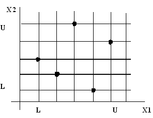
In the Latin Hypercube technique the design space for each factor is divided uniformly (the same number of divisions, , for all factors). These levels are randomly combined to specify points defining the design matrix (each level of a factor is studied only once). For example, the following figure illustrates a possible Latin Hypercube configuration for two factors () in which five points are studied. While not as visually obvious, this concept easily extends to multiple dimensions.

An advantage of using the Latin Hypercube technique over the Orthogonal Arrays technique is that more points and more combinations can be studied for each factor. The Latin Hypercube technique allows the designer total freedom in selecting the number of designs to run (as long as it is greater than the number of factors). The configurations are more restrictive using the Orthogonal Arrays technique (L4, L8, etc.).
A drawback to the Latin Hypercubes are that they are not reproducible because they are generated with random combinations. In addition, as the number of points decreases, the chances of missing some regions of the design space increases.