General Linear Equation Calculations

The relationship between the response and signal factor for this case can be modeled as $y=m+\beta \left(M-\overline{M}\right)+e$

where $y$ is the response, $m=\overline{y}$, $M$ is the signal factor, $\overline{M}$ is the average of the signal factor levels, and $\beta$ is the slope of the line fit to the signal/response data, and $e$ is the error in this fit.

The dynamic signal-to-noise ratio is calculated for the general linear equation relationship as follows:

$r_0$ = number of noise experiments

$k$ = number of signal factor levels

1. Calculate the slope, $\beta$:
   $$\beta =\frac{1}{r}\left(\left(M_1-\overline{M}\right)y_1+\left(M_2-\overline{M}\right)y_2+\dots +\left(M_k-\overline{M}\right)y_k\right)$$

   where

   $$\text{r}={\text{r}}_0\left({\left(M_1-\overline{M}\right)}^2+{\left(M_2-\overline{M}\right)}^2+\dots +{\left(M_k-\overline{M}\right)}^2\right)$$
   $$\overline{M}=\frac{\left(M_1+M_2+\dots +M_k\right)}{k}$$

   and $y_k$ is the sum of the response values at signal level $k$.

2. Calculate the total sum of the squares:
   $$S_T=y_{11}^2+y_{12}^2+\dots +y_{k{r}_0}^2-\frac{{\left({\displaystyle \sum _{i=1}^k{\displaystyle \sum _{j=1}^{r_0}{y}_{ij}}}\right)}^2}{k{r}_0}$$
3. Calculate the variation caused by the linear effect:
   $$S_{\beta }=\frac{1}{r}{\left(\left(M_1-\overline{M}\right)y_1+\left(M_2-\overline{M}\right)y_2+\dots +\left(M_k-\overline{M}\right)y_k\right)}^2$$
4. Calculate the variation associated with error and nonlinearity:
   $$S_e=S_T-S_{\beta }$$
5. Calculate the error variance:
   $$V_e=\frac{1}{k{r}_0-2}{S}_e$$
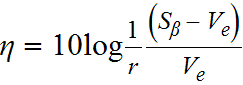
6. Calculate the dynamic $S/N$ ratio:

   

While the dynamic signal-to-noise ratio is used to measure the linearity of the signal-response relationship and the variability around this relationship, a sensitivity metric is used to measure the effect of the control experiments on the slope of this linear relationship. For a dynamic system, sensitivity is measured as follows:

A main effects analysis on this measure of sensitivity can be used to determine which control factors drive the slope of the signal-response relationship and ideally those that affect this sensitivity more than the dynamic signal-to-noise ratio can be used to adjust the system to the desired slope.